Everything on this page runs on runEDDB’s built-in GFN2-xTB engine: a plain .xyz geometry is all you need, and every command finishes in seconds. Start with the video for the 5-minute overview, pick a worked example below, and keep the cheat-sheet at the bottom open while you work.
Quick start in five minutes (video)
Quick-start video — coming soon
download → install → a crystal-structure geometry → EDDB, BDF and NICS-xTB in five minutes
The tutorials build on each other, but each one is self-contained: every geometry and every output is on its page.
◼ Command cheat-sheet
The commands you will use most often, on a molecule everybody knows: the built-in benzene model, -i @benzene, which needs no file at all (see the note below). Prefer a file? Download benzene.xyz (an idealized D6h geometry, same atom numbering) and write -i benzene.xyz instead. Swap in your own file and atom numbers for real work. Below the commands, a compact reference to the three things you steer on every run: what to analyse (scope), what to report (tables), and what to export for visualization.
runEDDB — the everyday commands
$ runEDDB -i @benzene -q # summary only (quiet)$ runEDDB -i @benzene --table npa # charges + populations$ runEDDB -i @benzene --export-cube eddb -n 4 # EDDB_G map (.cube), 4 cores$ runEDDB -i @benzene --export-cube bdf -a # signed π-BDF map$ runEDDB -i @benzene -p 1-2-3-4-5-6-1 -a --table npa # ring CDI (π only)$ runEDDB -i @benzene -r 6 # find rings → benzene.rings$ runEDDB -i @benzene --export-fchk nobd -a --table nobd # π-NOBDs as .fchk$ runEDDB -i @benzene --cite both # references for this run$ runEDDB -i @list # built-in model catalogue$ runEDDB -i benzene.fchk # ab-initio wavefunction instead
About @benzene. runEDDB ships a built-in library of test geometries, so every command above works without any file at hand — the same goes for @naphthalene, @pyrrole, @coronene, @porphine and some 30 more (runEDDB -i @list prints the catalogue). Ring atoms are numbered consecutively, heteroatom first (pyrrole: N1, C2–C5), so a pathway like 1-2-3-4-5-6-1 means what you expect; for fused rings use -r to get the strings. The library geometries are force-field conformers meant for testing — for real work use your own optimized structure, e.g. the benzene.xyz above. Windows PowerShell users: quote the name, -i '@benzene', because a bare @ is PowerShell’s splatting operator (in cmd.exe no quotes are needed).
1 · Choose what to analyse — the five scope modes (-g / -h / -f / -p / -r)
One mutually-exclusive flag selects the region of delocalization the analysis (and any exported cube) focuses on. They are the backbone of an EDDB study:
--global / -g — EDDBG: the whole molecule (the default). The global delocalization picture.
--heavy-atoms / -h — EDDBH: the whole molecule like EDDBG, but every connection to a hydrogen is dropped from the connectivity before the analysis. The natural sibling of EDDBG (and the scope recommended as default in the legacy runEDDB.R): faster on large π-conjugated systems, and it keeps C–H hyperconjugation out of the π-NOBD picture (no σ/π mixing). (Note: -h is this scope, not help — use --help.)
--fragment / -f LIST — EDDBF: restrict the populations / cube to a chosen set of atoms, e.g. -f 1:6,10,12 — the rest of the molecule is still fully present in the wavefunction.
--pathway / -p CHAIN — EDDBP: a specific cyclic pathway, e.g. -p 1-2-3-4-5-6-1 (repeat the first atom to close the ring). This is how you get the Cyclic Delocalization Index (CDI) — a direct, quantitative aromaticity measure.
--ring-detect / -r LIST — EDDBR: automatically find every n-membered ring (sizes you ask for, e.g. -r 6 or -r 5,6,7) in the bond-order graph and run a CDI on each — an automatic -p over the whole molecule, with the full ring list written to <stem>.rings.
See §3 Analysis Modes for the full details (plus NOBD dissection and the NAO basis subsets).
2 · Read the bonding — universal analysis tables (--table)
These print straight to the terminal — no file written — and are powerful, universal one-liners that work on any wavefunction the program can read. Two of them stand out:
--table npa — Natural Population Analysis: natural atomic charges qN (ECP- and GFN2-aware), orbital- and condensed-atomic populations, and the per-atom electron delocalization. A complete, NBO-quality population analysis from any input.
--table bo — Bond-Order Orbitals: each pair’s (Wiberg) bond order resolved into orthonormal bond-order orbitals, each carrying a σ/π/δ/φ symmetry label — a spin- and correlation-consistent generalisation of the bond index, the textbook way to see what a bond is made of. (Aliases boo / nba are accepted; add --export-fchk bo to write the orbitals for viewing.)
(--table no adds the natural-orbital occupancy table, with its multireference / spin-contamination indices shown under -v; --table nobd the NOBD-resolution table; --table mo the per-MO ED / EDLB / EDDB decomposition when canonical MOs are present; --table all emits everything.) For example, what a benzene C–C bond is actually made of — one command:
runEDDB -i benzene.fchk --table bo
  ┌────────────────────────────────────────────────────────────────────────────────────┐
  │                       BOND-ORDER ORBITALS (BOO) IN NVB BASIS                       │
  └────────────────────────────────────────────────────────────────────────────────────┘
    Index      Atom pair         Total        BOO occupations with symmetry labels
   ─────── ─────────────────   ─────────  ─────────────────────────────────────────────
        1      1~2      C~C     1.44010    0.97498(σ) 0.44444(π) 0.01997(π) 0.00071(σ)
        5      1~4      C~C     0.11731    0.11111(π) 0.00383(σ) 0.00236(π)
        8      1~6      C~C     1.44010    0.97498(σ) 0.44444(π) 0.01997(π) 0.00071(σ)
       12      1~7      C~H     0.97256    0.97256(σ)
        … (atoms 2–6 repeat the same C–C and C–H pattern)
   ─────── ─────────────────   ─────────  ─────────────────────────────────────────────
    (σ/π/δ/φ = bond-orbital symmetry; Total = full Wiberg index over all BOOs)

  Each row leads with the global Index of the pair’s first BOO (its last is implicit
  — one below the next row’s Index — and matches the MO numbering of --export-fchk bo).
  Each aromatic C–C bond resolves into 0.975 σ + 0.444 π — the π piece is
  exactly the delocalized component EDDB maps; the weak 1–4 "meta" interaction
  is pure π; every C–H is a single σ.
3 · Export for visualization (--export-cube / --export-fchk)
Write Gaussian .cube volumetric fields (ed, eddb, edlb, bdf, their differential maps, and per-orbital cubes via ao|no|nobd|bo|xtb[LIST] — one exactly-evaluated cube per selected orbital, faithful in any viewer) or Gaussian .fchk orbitals (nobd, no, bo, the ao basis set, or the GFN2-xTB wavefunction) for any cube/FCHK viewer. Each verb takes a comma-separated list, so one call can emit many coherent files at once. See §5 Output Files and §6 Differential Maps.
Where to go next. The full reference lives in the Manual: §2 covers every input format and the built-in GFN2-xTB engine; §3 the analysis modes; §4 every command-line option; §5–§7 the outputs and how to read them.
4 · Feed an ab-initio wavefunction (--input FILE)
GFN2-xTB is a fast first pass. For publication-quality numbers, run a single point in your quantum-chemistry program and hand the wavefunction file to runEDDB — the analysis is identical regardless of the source program; only the way you generate the file differs. The inputs below all run benzene at the CAM-B3LYP/cc-pVDZ level (a long-range-corrected functional, important for a balanced description of delocalization; cc-pVDZ is built into every program listed, so the inputs stay short and comparable). Each block is one program — expand the one you use.
Gaussian 16
The route section requests a checkpoint, which formchk converts to a formatted one (tested: ES64L-G16RevC.01). Input file: 💾 benzene.gjf.
benzene.gjf
%Chk=benzene.chk
#P CAM-B3LYP/cc-pVDZ

benzene, CAM-B3LYP/cc-pVDZ single point for runEDDB

0 1
C         1.39100000       0.00000000       0.00000000
C         0.69550000       1.20464134       0.00000000
C        -0.69550000       1.20464134       0.00000000
C        -1.39100000       0.00000000       0.00000000
C        -0.69550000      -1.20464134       0.00000000
C         0.69550000      -1.20464134       0.00000000
H         2.47400000       0.00000000       0.00000000
H         1.23700000       2.14254685       0.00000000
H        -1.23700000       2.14254685       0.00000000
H        -2.47400000       0.00000000       0.00000000
H        -1.23700000      -2.14254685       0.00000000
H         1.23700000      -2.14254685       0.00000000
After the SCF, convert the binary benzene.gbw to the JSON wavefunction format with orca_2json (tested: 6.0.1); runEDDB reads benzene.json directly. Input file: 💾 benzene.inp.
benzene.inp
! CAM-B3LYP cc-pVDZ
* xyz 0 1
C         1.39100000       0.00000000       0.00000000
C         0.69550000       1.20464134       0.00000000
C        -0.69550000       1.20464134       0.00000000
C        -1.39100000       0.00000000       0.00000000
C        -0.69550000      -1.20464134       0.00000000
C         0.69550000      -1.20464134       0.00000000
H         2.47400000       0.00000000       0.00000000
H         1.23700000       2.14254685       0.00000000
H        -1.23700000       2.14254685       0.00000000
H        -2.47400000       0.00000000       0.00000000
H        -1.23700000      -2.14254685       0.00000000
H         1.23700000      -2.14254685       0.00000000
*
Turbomole has no single input file. Put the 💾 coord file (Cartesian coordinates in Bohr) in an empty directory and let define build control, basis and the start orbitals. The whole interactive session can be driven by piping the answers on stdin (cc-pVDZ on all atoms, CAM-B3LYP via libxc, default charge and occupations):
coord
$coord  natoms=    12
    2.62860903931860     0.00000000000000     0.00000000000000      c
    1.31430451965930     2.27644221097115     0.00000000000000      c
   -1.31430451965930     2.27644221097115     0.00000000000000      c
   -2.62860903931860     0.00000000000000     0.00000000000000      c
   -1.31430451965930    -2.27644221097115     0.00000000000000      c
    1.31430451965930    -2.27644221097115     0.00000000000000      c
    4.67518243226040     0.00000000000000     0.00000000000000      h
    2.33759121613020     4.04882675562444     0.00000000000000      h
   -2.33759121613020     4.04882675562444     0.00000000000000      h
   -4.67518243226040     0.00000000000000     0.00000000000000      h
   -2.33759121613020    -4.04882675562444     0.00000000000000      h
    2.33759121613020    -4.04882675562444     0.00000000000000      h
$end
terminal
$ echo -e "\nbenzene\na coord\n*\nno\nb all cc-pVDZ\n*\neht\ny\n0\ny\ndft\non\nfunc hyb_gga_xc_cam_b3lyp\n*\n*\n" | define
Then run the SCF and concatenate control + coord + basis + mos into a single .tmol bundle that runEDDB reads directly:
terminal
$ dscf && cat control coord basis mos > benzene.tmol
$ runEDDB --input benzene.tmol
Other accepted inputs: Molden files (.molden) and NBO7 archive files (.49); see §2 of the Manual for the full list and the fine print of each format.