◼ Tutorial 2 — Phenanthrene: Clar’s rule made visible
Phenanthrene has three fused six-membered rings. Are they equally aromatic? Clar’s rule says no — and in this tutorial runEDDB shows you why, in three steps: it finds the rings for you, gives each a CDI, and draws a 3D map that tells delocalized bonds from localized ones.
What you will learn
Using -r (or --ring-detect) to detect every ring of a chosen size automatically — no atom indices to type.
Running the pathway analysis on each detected ring in one shell loop and collecting the CDIs.
Computing the Bond Delocalization Function (BDF) and exporting it as a 3D map.
Looking at the Natural Orbitals for Bond Delocalization (NOBD) to check what the automatic π-selection picked.
Reading the results in terms of Clar’s rule.
Before you start
Download the geometry. As in Tutorial 1, the input is a plain .xyz file, so runEDDB builds the wavefunction itself with its built-in GFN2-xTB engine; every run takes a second or two.
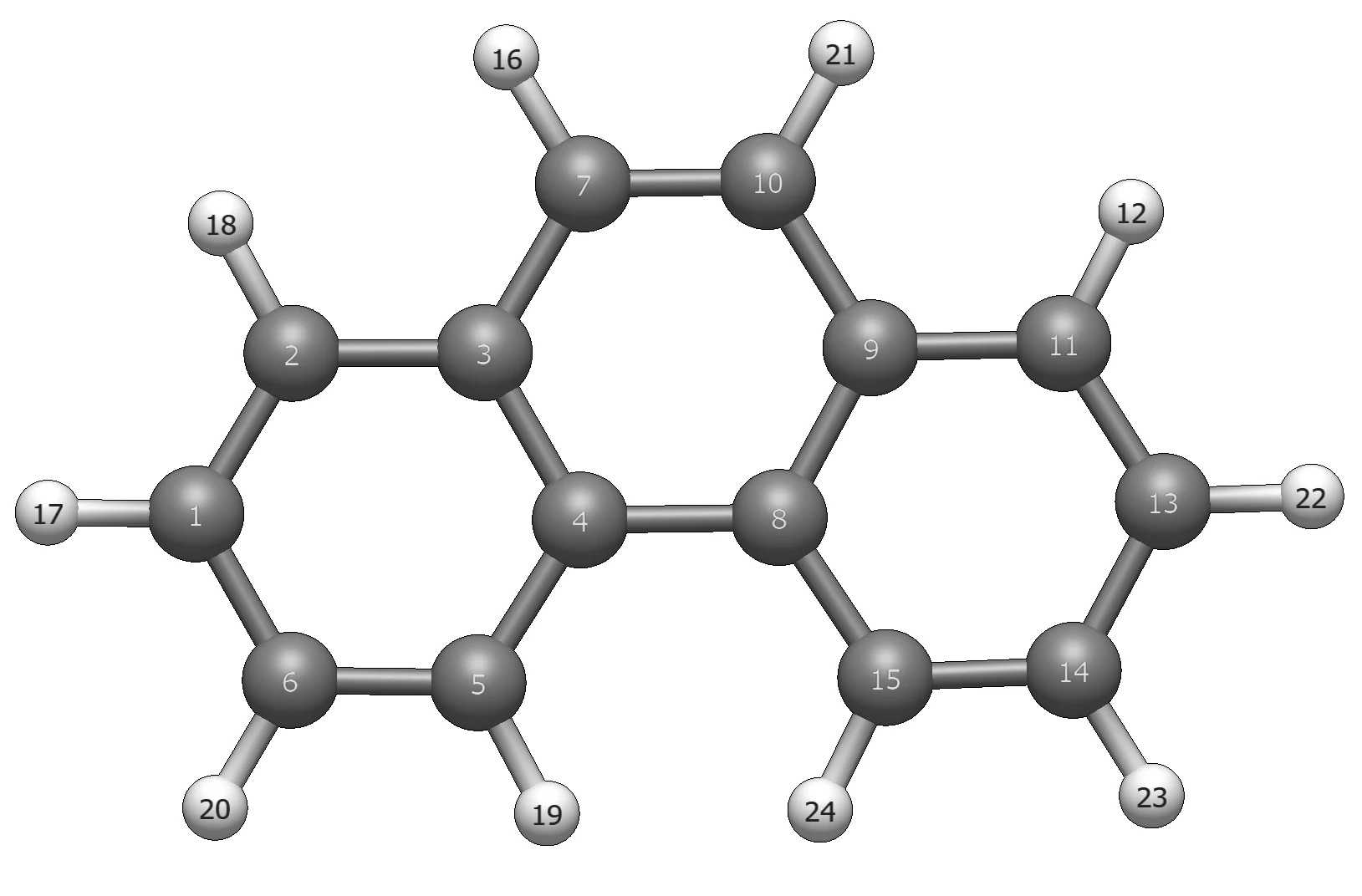
Phenanthrene with the atom numbering of phenanthrene.xyz.
(A phenanthrene model is also built into runEDDB, -i @phenanthrene, but with a different geometry and atom order; use the file above so that your numbers match this page.)
We want the CDI of each ring. To get it we have to tell runEDDB which atoms form each ring — and for a polycyclic molecule, writing pathway strings by hand quickly becomes tedious and error-prone. runEDDB can do it for you.
Part 1 — Finding the rings automatically
terminal
$ runEDDB -i phenanthrene.xyz -r 6
-r 6 (or --ring-detect 6) searches the bond-order graph for six-membered rings. Several sizes can be requested at once: -r 5:8 covers 5- to 8-membered rings, -r 5,6 just those two.
output
────────────────────────────────────────────────────────────────────────────────────────
                                ▄▄▄▄▄▄▄▄▄▄▄▄▄▄▄▄▄▄▄▄▄▄▄▄▄                    Build date:
                              r █▄ ▄▄ █▄ ▄▄▀█▄ ▄▄▀█▄ ▄ ▀█                    2026-Sep-15
                              u ██ ▄█▀██ ██ ██ ██ ██ ▄ ▀█
                              n █▄▄▄▄▄█▄▄▄▄██▄▄▄▄██▄▄▄▄██

                     Electron Density of Delocalized Bonds Analysis
                        (https://aromaticity.uj.edu.pl/runeddb)
────────────────────────────────────────────────────────────────────────────────────────

▶ Loading and parsing input file...                                                   0s
▶ Modelling one-electron density at the GFN2-xTB/vSTO-nG level...                     0s
▶ Building natural atomic orbitals (NAO, frozen-NMB two-cycle)...                     0s
▶ Exporting detected rings (3) to phenanthrene.rings...                               0s
▶ Performing multicenter bond-orbital projections (BOP)...                            0s
▶ Computing natural orbitals for bond delocalization (NOBD)...                        0s
▶ Printing summary of EDDB calculations:

        Total   ED_R population:           56.10556    per atom:     4.00754
        Total EDLB_R population:           46.69254    per atom:     3.33518
        Total EDDB_R population:            9.41302    per atom:     0.67236

▶ Calculation completed on 2026-09-17. Total time: 0s.
The detected rings are written to phenanthrene.rings:
The header records the search criteria: the ring sizes requested and the bond-order cutoff used to decide which contacts count as ring bonds (0.30 by default, adjustable with --ring-thresh). Three rings were found; their atom indices are listed at the bottom, one -p pathway string per line, ready to be fed straight back into runEDDB.
Part 2 — The CDI of every ring
The # per-ring CDI line of the .rings file is a ready-made shell loop. Fill in the two placeholders (FILE → phenanthrene.rings, INPUT → phenanthrene.xyz), add a label line so you know which ring is which, and run it:
terminal
$ grep -v '^#' phenanthrene.rings | while read -r r; do echo "== ring $r"; runEDDB -i phenanthrene.xyz -p "$r" -a -q -c 0; done &> phenanthrene-cdi.log
⚠ Add -a yourself. The loop suggested in the .rings file does not include it. Without -a the analysis covers all valence electrons, so the CDI would mix σ- and π-delocalization and would not be the π-aromaticity index you want to report.
What the rest of the loop does: -p "$r" runs the pathway analysis on one ring per iteration; -q prints only the summary; -c 0 disables cube writing (nothing is exported here anyway, but it keeps the directory clean); &> phenanthrene-cdi.log sends everything to one log file.
phenanthrene-cdi.log
== ring 1-2-3-4-5-6-1

────────────────────────────────────────────────────────────────────────────────────────
                                ▄▄▄▄▄▄▄▄▄▄▄▄▄▄▄▄▄▄▄▄▄▄▄▄▄                    Build date:
                              r █▄ ▄▄ █▄ ▄▄▀█▄ ▄▄▀█▄ ▄ ▀█                    2026-Sep-15
                              u ██ ▄█▀██ ██ ██ ██ ██ ▄ ▀█
                              n █▄▄▄▄▄█▄▄▄▄██▄▄▄▄██▄▄▄▄██

                     Electron Density of Delocalized Bonds Analysis
                        (https://aromaticity.uj.edu.pl/runeddb)
────────────────────────────────────────────────────────────────────────────────────────

▶ Printing summary of EDDB calculations:

        Total   ED_P population:            5.99556    per atom:     0.99926
        Total EDLB_P population:            2.10869    per atom:     0.35145
        Total EDDB_P population:            3.88687    per atom:     0.64781

    Cyclic Delocal. Index (CDI):            0.51863
    Delocalized fraction (%del):              64.83 %
    Cyclic coherence (%cyc):                  51.90 %

▶ Calculation completed on 2026-09-17. Total time: 0s.

== ring 3-4-8-9-10-7-3

────────────────────────────────────────────────────────────────────────────────────────
                                ▄▄▄▄▄▄▄▄▄▄▄▄▄▄▄▄▄▄▄▄▄▄▄▄▄                    Build date:
                              r █▄ ▄▄ █▄ ▄▄▀█▄ ▄▄▀█▄ ▄ ▀█                    2026-Sep-15
                              u ██ ▄█▀██ ██ ██ ██ ██ ▄ ▀█
                              n █▄▄▄▄▄█▄▄▄▄██▄▄▄▄██▄▄▄▄██

                     Electron Density of Delocalized Bonds Analysis
                        (https://aromaticity.uj.edu.pl/runeddb)
────────────────────────────────────────────────────────────────────────────────────────

▶ Printing summary of EDDB calculations:

        Total   ED_P population:            5.97348    per atom:     0.99558
        Total EDLB_P population:            4.33594    per atom:     0.72266
        Total EDDB_P population:            1.63754    per atom:     0.27292

    Cyclic Delocal. Index (CDI):            0.26855
    Delocalized fraction (%del):              27.41 %
    Cyclic coherence (%cyc):                  26.97 %

▶ Calculation completed on 2026-09-17. Total time: 0s.

== ring 8-9-11-13-14-15-8

────────────────────────────────────────────────────────────────────────────────────────
                                ▄▄▄▄▄▄▄▄▄▄▄▄▄▄▄▄▄▄▄▄▄▄▄▄▄                    Build date:
                              r █▄ ▄▄ █▄ ▄▄▀█▄ ▄▄▀█▄ ▄ ▀█                    2026-Sep-15
                              u ██ ▄█▀██ ██ ██ ██ ██ ▄ ▀█
                              n █▄▄▄▄▄█▄▄▄▄██▄▄▄▄██▄▄▄▄██

                     Electron Density of Delocalized Bonds Analysis
                        (https://aromaticity.uj.edu.pl/runeddb)
────────────────────────────────────────────────────────────────────────────────────────

▶ Printing summary of EDDB calculations:

        Total   ED_P population:            5.99556    per atom:     0.99926
        Total EDLB_P population:            2.10868    per atom:     0.35145
        Total EDDB_P population:            3.88688    per atom:     0.64781

    Cyclic Delocal. Index (CDI):            0.51863
    Delocalized fraction (%del):              64.83 %
    Cyclic coherence (%cyc):                  51.90 %

▶ Calculation completed on 2026-09-17. Total time: 0s.
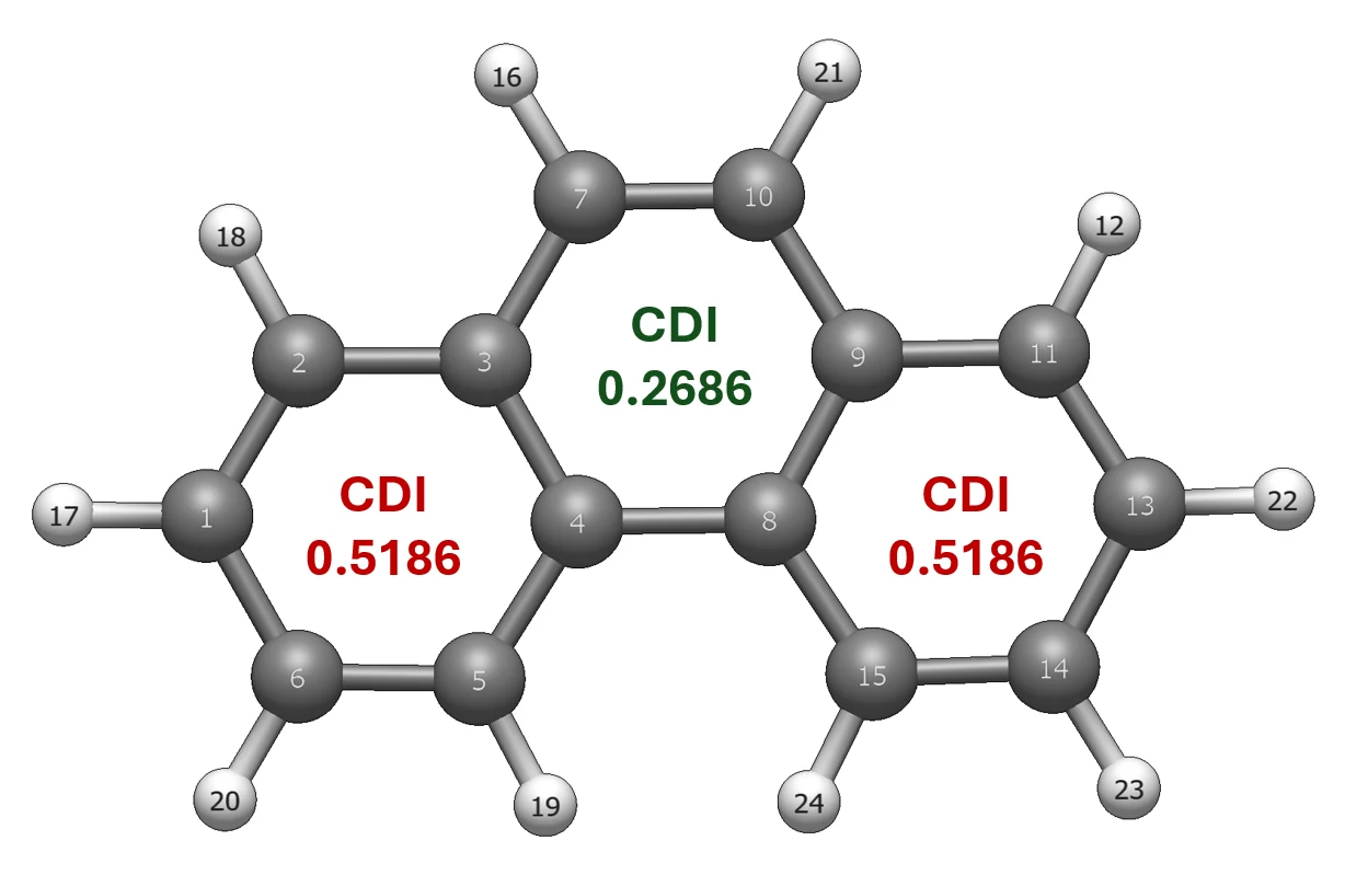
CDI of each ring, on the atom numbering of phenanthrene.xyz.
The two terminal rings reach CDI = 0.519 e per atom, while the central ring manages only 0.269. Cyclic delocalization is far more efficient in the terminal rings — in line with what other aromaticity indices (HOMA, NICS) say about phenanthrene.
Part 3 — The Bond Delocalization Function (BDF)
The EDDB decomposition splits the electron density into a delocalized part (EDDB) and a localized part (EDLB). Their difference, restricted to the π-electrons,
BDFπ = EDDBπ − EDLBπ
is a signed 3D function: BDF > 0 marks regions where delocalization dominates, BDF < 0 marks localized bonds, and BDF ≈ 0 means the two are comparable. It is the one map that can show a localized bond next to delocalized ones.
terminal
$ runEDDB -i phenanthrene.xyz --export-cube bdf -a
--export-cube bdf writes the map to phenanthrene.BDF_G.cube; -a restricts it to the π-electrons.
output
────────────────────────────────────────────────────────────────────────────────────────
                                ▄▄▄▄▄▄▄▄▄▄▄▄▄▄▄▄▄▄▄▄▄▄▄▄▄                    Build date:
                              r █▄ ▄▄ █▄ ▄▄▀█▄ ▄▄▀█▄ ▄ ▀█                    2026-Sep-15
                              u ██ ▄█▀██ ██ ██ ██ ██ ▄ ▀█
                              n █▄▄▄▄▄█▄▄▄▄██▄▄▄▄██▄▄▄▄██

                     Electron Density of Delocalized Bonds Analysis
                        (https://aromaticity.uj.edu.pl/runeddb)
────────────────────────────────────────────────────────────────────────────────────────

▶ Loading and parsing input file...                                                   0s
▶ Modelling one-electron density at the GFN2-xTB/vSTO-nG level...                     0s
▶ Building natural atomic orbitals (NAO, frozen-NMB two-cycle)...                     0s
▶ Performing multicenter bond-orbital projections (BOP)...                            0s
▶ Computing natural orbitals for bond delocalization (NOBD)...                        0s
▶ Exporting BDF_G to phenanthrene.BDF_G.cube...                                       1s
▶ Printing summary of EDDB calculations:

        Total   ED_G population:           14.00000    per atom:     0.58333
        Total EDLB_G population:            3.99165    per atom:     0.16632
        Total EDDB_G population:           10.00835    per atom:     0.41701

▶ Calculation completed on 2026-09-17. Total time: 1s.
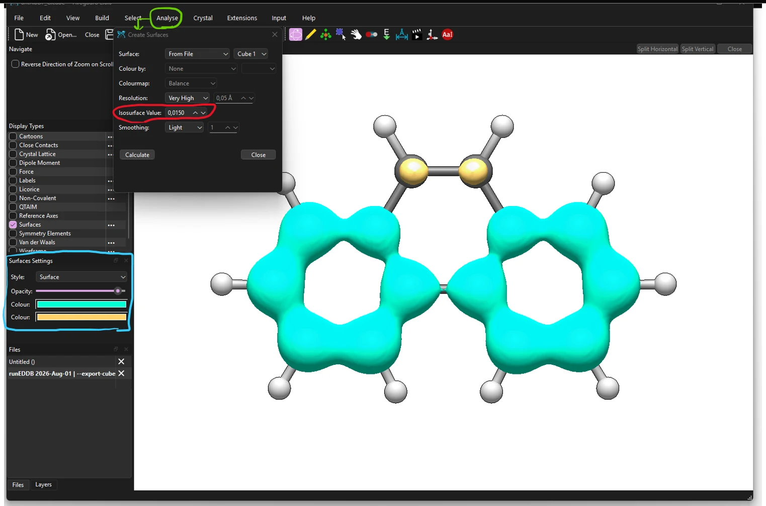
Open the cube in Avogadro2: Analyze → Create Surfaces (green), set the isovalue (red), and — because BDFπ is signed — give the positive and negative lobes two contrasting colours in the Surface Settings panel (blue):
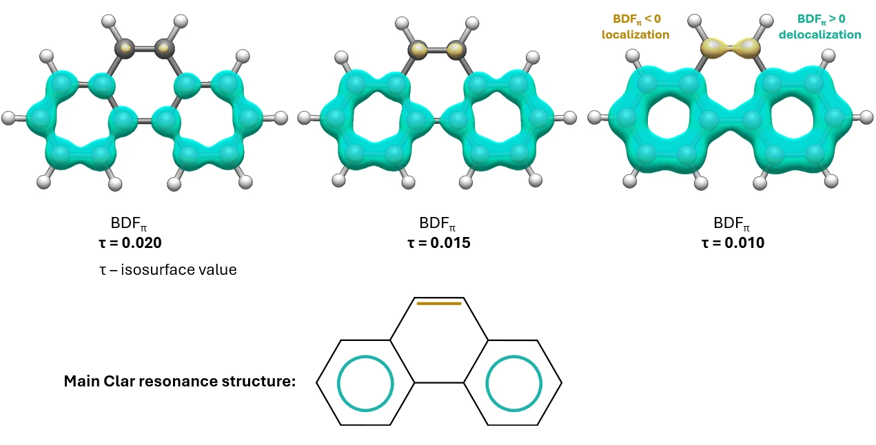
BDFπ of phenanthrene at three isovalues. Cyan: delocalized (BDF > 0); yellow: localized (BDF < 0). Bottom: the main Clar resonance structure.
Clar’s rule states that the dominant resonance structure of a polycyclic aromatic hydrocarbon is the one with the largest number of disjoint aromatic π-sextets. The BDFπ map reproduces this directly: two isolated π-sextets sit in the terminal rings, while the central C=C bond (atoms 7–10) shows up as a localized double bond. Placing the sextets in the terminal rings forces that bond to localize — exactly the main Clar structure.
Part 4 — Looking at the NOBDs
The Natural Orbitals for Bond Delocalization are the orbitals that carry the delocalized density. -a chooses the π-type ones automatically — and this is where you check that it chose well.
terminal
$ runEDDB -i phenanthrene.xyz --export-fchk nobd -a --table nobd
--export-fchk nobd writes the NOBDs to phenanthrene.NOBD_G.fchk, so they can be visualized like ordinary molecular orbitals; --table nobd prints the NOBD table (runEDDB prints tables only when asked).
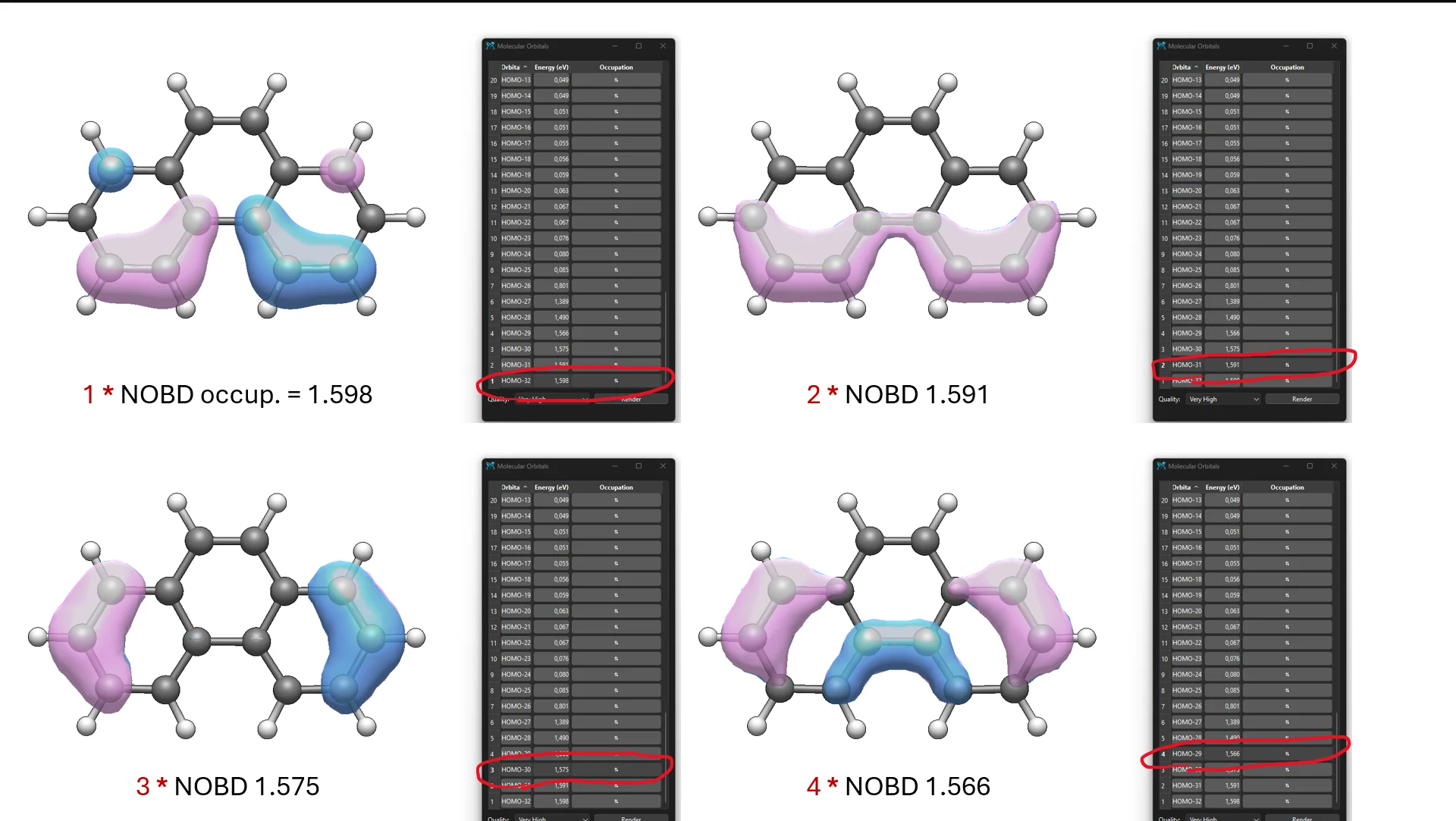
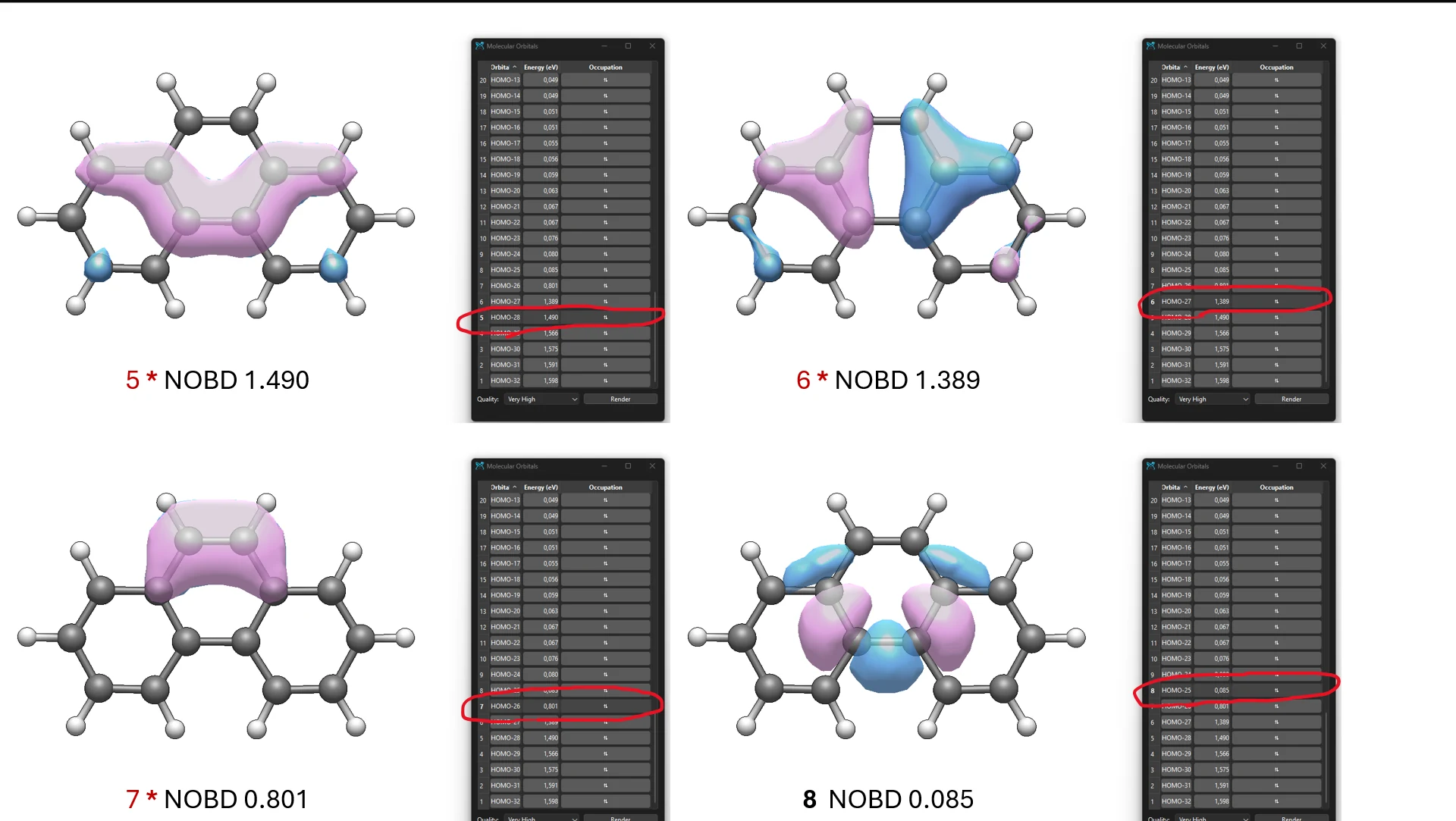
NOBDs are listed by decreasing occupancy, so the largest contributors to delocalization come first. The ones selected by -a carry a star in the Sel column; the s, p, d, f columns give the contribution of each orbital type. Phenanthrene has 14 π-electrons and seven NOBDs are selected as π — each built entirely from carbon 2p orbitals (%p = 100). The occupancy of the 8th NOBD drops to 0.085, about ten times less than the 7th, the last one selected.
Occupancies are delocalization eigenvalues, not orbital populations. The seven starred values add up to 10.008 e — exactly the Total EDDB_G printed in the summary, not the 14 π-electrons of Total ED_G. Roughly 72% of the π-density is delocalized; the remaining 3.99 e is localized.
To see the NOBDs, open phenanthrene.NOBD_G.fchk in any program that renders orbitals from FCHK files — here Avogadro2. The first NOBD sits at the bottom of the orbital list (labelled 1 HOMO-32); reading upwards, occupancy and contribution to delocalization decrease. The Energy (eV) column does not hold energies — it holds each NOBD’s occupancy, the same numbers as in the table.
NOBDs 1–4, all selected as π.
NOBDs 5–8. The eighth is not starred — and indeed it is a σ-orbital.
The shapes confirm that the first seven NOBDs are of π-symmetry and that NOBD 8 is σ: --auto-pi separated them correctly. On more complex molecules, or whenever a result looks suspicious, look at the NOBDs before trusting the dissection.
What to try next
Export --export-cube eddb,edlb,bdf in a single run and compare the three maps side by side. EDDB alone cannot show a localized bond — only the signed BDF can.
Add --cite both to any run: runEDDB prints the exact reference list for the methods that run actually used.
Try -r 5:7 on a molecule with rings of different sizes and look at the .rings file.
Where to go next.Tutorial 3 takes on a harder case — a metallacycle where the automatic π-selection deserves a second look. The cheat-sheet collects every command in one place, and the Manual is the full reference.