Electron Density of Delocalized Bonds (EDDB)

Szczepanik Research Group

Department of Theoretical Chemistry
Faculty of Chemistry, Jagiellonian University
Gronostajowa 2, 30-387 Krakow, Poland
Tel: (+48) 12 686 23 90
E-mail: dariusz.szczepanik@uj.edu.pl

HOME PROJECTS PUBLICATIONS runEDDB molANO X

About EDDB/BDF Download Tutorials Manual

◼ What makes aromatic delocalization special

Electron delocalization is one of the most fundamental concepts in chemistry. In its broadest sense, it refers to the spreading of electron density over a region larger than a single atom or a single bond. Yet not all forms of delocalization are alike, and understanding the differences is essential if one wants to characterize aromatic and conjugated systems in a chemically meaningful way.

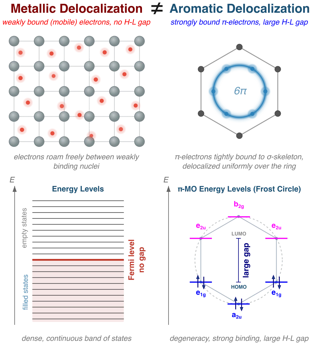
Consider, for example, the delocalization that occurs in metallic solids. The outermost valence electrons of a metal sit near the Fermi level and are only weakly bound to any particular nucleus. They move with relatively high kinetic energy through the lattice, hopping easily from site to site. It is precisely this high mobility—the ease with which electrons can be transferred through the network—that gives metals their characteristic electrical conductivity. In this regime, “delocalized” is essentially synonymous with “mobile” and “loosely bound.”

The π-electron system of benzene could hardly be more different. On a superficial level, it too is called delocalized: the six π-electrons are spread uniformly over the ring rather than being confined to three alternating double bonds. Yet the physical origin of this delocalization is not weak binding, but its opposite. The cyclic topology of the six carbon nuclei creates a pattern of one-electron energy levels that is qualitatively distinct from the pattern found in an open-chain analogue such as hexatriene. Specifically, the cyclic arrangement introduces a degeneracy of π-molecular-orbital levels (the well-known Frost–Musulin mnemonic makes this visible at a glance), which has three interrelated consequences:

The π-electrons fill into levels that lie lower in energy than the corresponding levels of the open chain. A direct comparison of the orbital energies of benzene and hexatriene shows that the occupied π-levels of benzene are noticeably more stable, meaning that the π-electrons are more tightly bound to the nuclear framework.
The highest occupied π-level (HOMO) is lowered while the lowest unoccupied level (LUMO) is raised, producing a larger HOMO–LUMO gap than in the open chain. A large gap implies high kinetic stability: the π-electrons sit in a deep potential well and are resistant to perturbation.
The degeneracy of the occupied π-levels enforces a uniform distribution of π-bonding around the ring—what may be called π-coherence. No single C–C bond carries more or less π-character than any other. This uniformity is the structural signature of aromaticity and contrasts sharply with the bond-length alternation typical of non-aromatic conjugated chains.

Taken together, these features lead to a situation that may seem counterintuitive at first: the π-electrons of benzene are simultaneously more delocalized and less mobile than those of a comparable open-chain system. They are spread over a wider region of the molecule (delocalized), yet they are harder to excite, harder to remove, and harder to engage in addition reactions (less mobile). The low kinetic energy and strong binding of the π-cloud is what makes benzene so characteristically unreactive toward electrophilic addition—a textbook property that sets aromatic systems apart from ordinary polyenes.

This distinction has an important conceptual consequence. In metals, one speaks naturally of “delocalized electrons”—individual electrons that are free to roam. In benzene, a more precise language is called for. What is delocalized is not so much the electrons themselves as the bonds they form: each π-bond is shared equally among all adjacent C–C pairs, creating a closed circuit of partial bonds rather than a set of free-roaming charges. In other words, the characteristic feature of aromatic delocalization is the delocalization of π-bonds, not merely of π-electrons.

Bond delocalization is a more specific concept than electron delocalization in general. It captures precisely the aspect of aromatic and conjugated systems that distinguishes them from metallic or free-electron delocalization: the spreading of well-defined, strongly bound bonding interactions over a network of atoms, accompanied by increased electron binding and decreased kinetic energy. The Electron Density of Delocalized Bonds (EDDB) method is designed to quantify exactly this type of delocalization.

◼ Electron Density of Delocalized Bonds (EDDB)

Once we accept that what is characteristic of aromatic and conjugated systems is the delocalization of bonds rather than of individual electrons, a natural question follows: how do we measure this effect from a quantum-chemical calculation? A variety of strategies have been proposed over the past decades, and they broadly fall into two families. The first family constructs a particular set of bonding orbitals — natural bond orbitals (NBO), adaptive natural density partitioning (AdNDP), localized molecular orbitals, and the like — and then interprets the molecule through that chosen representation. The second family avoids orbitals altogether and works directly in three-dimensional physical space, analyzing the topology of the electron density itself (QTAIM, ELF, and related schemes). Both perspectives have been enormously productive, but each embeds a methodological choice that can blur the question at hand. Orbital-based approaches inevitably depend on the particular bonding representation one has decided to adopt; topological methods, in turn, describe where the density is but have difficulty quantifying which part of it is engaged in orbital conjugation.

The EDDB method takes a deliberately different stance. Its aim is not to define yet another orbital representation of bonding and not to classify points in space, but to isolate directly within the one-electron density matrix the fraction of the electron density that is participating in multi-centre, conjugated bonding. Bond orbitals still appear in the procedure, but only as auxiliary mathematical tools — a convenient probe used to interrogate the density matrix. The object that is finally reported — a density, visualizable in real space and integrable to an electron count — belongs unambiguously to the density itself and carries no arbitrariness inherited from a chosen orbital localization scheme. In this sense, EDDB sits at the intersection of the two traditions: it uses orbital logic where orbital logic is informative (namely, to detect conjugation), and returns a density where a density is more robust (namely, for visualization, population analysis, and comparison across methods).

The physical idea behind the method is simple. If a bond orbital between atoms A and X is genuinely coupled — through a shared atom X — to an adjacent bond orbital between X and B, then the two bonds share some of their electron density. If instead the relative phases of the two bond orbitals cancel out, the bonds are electronically independent in spite of being geometrically contiguous. The first situation is conjugation; the second is what one observes in a non-conjugated chain of isolated double bonds. The EDDB method diagnoses each bond orbital in the molecule, identifies the fraction that is coupled to its neighbours, and accumulates exactly that fraction into a new density matrix — the density of delocalized bonds. The remainder, by construction, carries the complementary electrons — those involved in localized bonds and lone pairs — and defines the Electron Density of Localized Bonds (EDLB).

◼ Numerical realization: the BOP algorithm

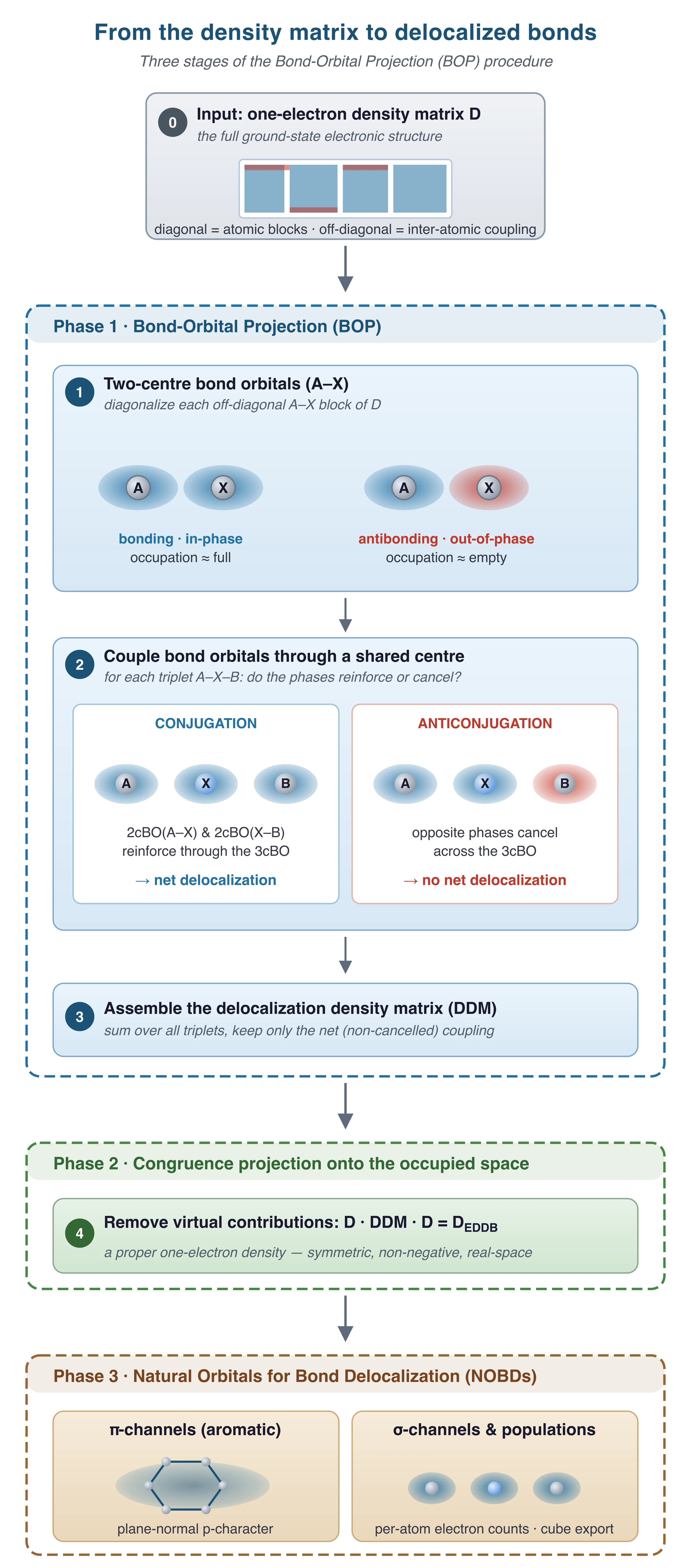
The practical machinery by which EDDB is extracted from the density matrix is the Bond-Orbital Projection (BOP) procedure. It proceeds in three logical stages, summarized in the figure on the right.

(i) Two-centre bond orbitals. For every pair of bonded atoms A and X the off-diagonal block of the one-electron density matrix, D(A,X), is diagonalized. The resulting eigenvectors form a set of two-centre bond orbitals (2cBOs), and their squared eigenvalues give the occupations of the bonding and anti-bonding components of the A–X bond. These orbitals play the role of “atomic orbitals” in the next step — they are the building blocks of bonding, one level up from AOs.

(ii) Three-centre coupling: conjugation versus anticonjugation. This is the defining step of the algorithm. For every triplet of bonded atoms A–X–B (where X is the shared centre), the corresponding triatomic block of D is diagonalized to yield a set of three-centre natural orbitals (3cBOs) spanning the A–X–B subspace. The two-centre orbitals built in stage (i) are then projected onto these 3cBOs, and the relative phases of the A–X and X–B projections are compared. When they reinforce each other the two bond orbitals conjugate (constructive interference — the essence of aromatic and polyenic delocalization). When they cancel, the bonds are effectively independent. This is the same logic that governs the formation of bonding and antibonding MOs in the diatomic case, only lifted one level higher: instead of atomic orbitals combining to form bonds, here bond orbitals combine to form delocalized conjugation channels. Summing over all triplets and keeping only the net, non-cancelled coupling yields a delocalization density matrix, DDM.

(iii) Projection onto the occupied space. DDM is defined in the full orbital space and in general contains contributions from virtual orbitals, which carry no physical electrons. A congruence transformation with the ground-state one-electron density matrix D,

D_EDDB = D · DDM · D

projects the delocalization matrix onto the space of occupied orbitals and produces D_EDDB, the Electron Density of Delocalized Bonds itself. It is a proper, symmetric, non-negative one-electron density, and its trace returns the total number of electrons engaged in multi-centre conjugation:

N_EDDB = Tr D_EDDB = ∑_i n_i

Diagonalization of D_EDDB yields a small set of Natural Orbitals for Bond Delocalization (NOBDs) with occupations n_i. A geometric test — fitting a local plane to the atoms that support each NOBD and measuring the p-character projected onto that plane’s normal — separates π-type channels from σ-type ones automatically, with no user input about the molecular orientation. The same symmetry-based logic detects δ-type channels relevant for transition-metal aromatic systems. Atomic EDDB populations — the number of delocalized electrons assigned to each atom — follow from the diagonal of D_EDDB in the natural-atomic-orbital basis, and the density itself can be exported to a cube file for direct visualization in real space.

EDDB therefore answers a specific, chemically well-posed question: how much of the electron density is engaged in conjugated, multi-centre bonding, and where in the molecule does it live? The bond orbitals used along the way are auxiliary probes, not the final answer; the final answer is the density D_EDDB together with the natural orbitals that diagonalize it. This is what makes the method representation-independent in spirit, directly comparable across levels of theory, and equally well-suited to the local analysis of individual conjugated bonds and to the global assessment of aromaticity in extended systems.

◼ Bond Delocalization Function (BDF)

The EDDB method carries a natural partner. Together with the density of delocalized bonds, the same BOP machinery returns the density of localized bonds and lone pairs — the Electron Density of Localized Bonds (EDLB). The two densities are additive and exhaustive: for any chosen subspace of the one-electron density (for instance the π-manifold), their sum recovers the full density of that subspace,

ED_π = EDDB_π + EDLB_π

Summing the two simply reproduces what we started with. Much more informative is their difference — a signed map that at each point in space tells us whether the π-density is dominated by delocalized, conjugated bonding or by localized, olefinic bonding. This is the Bond Delocalization Function:

BDF_π = EDDB_π − EDLB_π = 2 · EDDB_π − ED_π

The sign tells the story:

Positive BDF — regions where delocalized π-density exceeds localized density. These are the aromatic circuits and Clar-type π-sextets, where electron density is genuinely shared across several bonds.
Negative BDF — regions where localized density prevails. These are the olefinic double bonds, where a well-defined two-centre π-bond carries most of the density.
Near-zero BDF — regions where the two components compensate. Far from being chemically uninteresting, these are the fingerprints of ionic resonance, charge-assisted delocalization, and competing bonding motifs (Kekulé vs.~quinoid, migrating π-sextets), phenomena that are notoriously hard to read off from the total π-density alone.

Visualized as a 3-D isosurface, BDF_π converts abstract talk of “resonance” into a concrete map one can inspect for any molecule: positive blue regions mark the aromatic domains, negative red regions mark the olefinic ones, and white gaps mark the compensation zones. No pre-specified resonance structure, no orbital localization choice, no arbitrary threshold: only the one-electron density matrix.

◼ Aromaticity and the response-theory detour

A word on why this matters. For several decades, aromaticity has been diagnosed almost exclusively by magnetic-response descriptors — NICS, ring currents, induced current densities (AICD, GIMIC) and their many variants. These techniques are elegant, experimentally well-calibrated, and extraordinarily useful. But they share one methodological feature that is rarely stated plainly: they do not describe the molecule’s ground state. They describe how the molecule responds to an external magnetic field.

Within the one-electron picture, that response is governed by a narrow subset of low-energy occupied-to-virtual excitations — typically a handful of frontier orbitals near the HOMO–LUMO gap. This was made quantitative by Fowler, Steiner and co-workers more than twenty years ago: the symmetry-based selection rules for ring currents pick out only a few frontier π-orbitals as current-carrying channels. The rest of the occupied π-manifold is essentially invisible to the magnetic probe. In short, magnetic descriptors measure a perturbative property of the electronic structure, filtered through a frontier-orbital lens.

This is not a criticism of magnetic-response methods — they are irreplaceable for what they do, and they are sensitive precisely because they focus on the most polarizable electrons. It is, however, a reason to be careful about what we mean when we say that a molecule “is aromatic”. By equating aromaticity with the strength of a ring current, the community has gradually transferred one of the oldest and most fundamental concepts of chemical bonding into the vocabulary of molecular response theory. The concept itself has thereby drifted away from its natural home — the theory of the chemical bond — and become an observable of molecular magnetochemistry.

In small, textbook-aromatic molecules like benzene the two perspectives agree: the frontier π-orbitals and the bulk of the π-density tell the same story. In large and topologically rich systems they need not. A porphyrin nanoring such as c-P12[b12] can support a global aromatic ring current (magnetic diagnosis: aromatic) while its ground-state π-density, revealed by BDF_π, is organized into twelve locally aromatic porphyrin subunits connected by olefinic linkers (bonding diagnosis: locally aromatic). Aza-supernaphthalene preserves nine Clar π-sextets even as oxidation progressively flips its magnetic classification. In the fused indacene dimer s-ID, the open-shell ground state trades one π-bond for two disjoint Clar sextets — a bonding reorganization that explains the OSS–CSS energy gap almost quantitatively, and that is visible in BDF_π but not in the current-density picture. The two descriptors are not contradictory; they are answering different questions.

Magnetic-response descriptors tell you what a molecule does when pushed by an external field; BDF tells you what a molecule is in the absence of any field. Both questions are legitimate and both answers are informative — but only the second belongs to the theory of chemical bonding. BDF was designed to return aromaticity to that native territory: a property of the ground-state electron density, readable directly from the wavefunction, free of resonance presuppositions, and comparable across levels of theory.

In practice, runEDDB produces EDDB_π, EDLB_π and BDF_π as separate cube files, ready for visualization in VMD, Chimera, Avogadro or any other molecular-graphics package. The full (all-electron) variants are available through the same command-line switches, and the π / σ / δ partitioning of every channel is performed automatically from the ground-state geometry. No separate localization step, no orbital editor, no follow-up calculation: the three maps are obtained in a single pass through the density matrix.

HOME PROJECTS PUBLICATIONS runEDDB molANO X