
Szczepanik Research Group
Department of Theoretical Chemistry
Faculty of Chemistry, Jagiellonian University
Gronostajowa 2, 30-387 Krakow, Poland
Tel: (+48) 12 686 23 90
E-mail: dariusz.szczepanik@uj.edu.pl
HOME PROJECTS PUBLICATIONS runEDDB X
About EDDB Download Tutorials Manual
Manual (2026-Nov-03)
runEDDB writes files only when you ask for them. Three verbs cover everything:
--export-cube for 3D fields on a grid (densities, orbitals, differences),
--export-map for 2D maps in a plane, and --export-fchk / --export-json
for orbitals that other programs can read. This page shows each with an example, explains the file names
and the grids, and ends with the differential maps that compare two systems.
1. What do you want to see?
| You want | Run |
|---|---|
| an isosurface of the delocalized (and the localized) density | runEDDB -i mol.fchk --export-cube eddb,edlb |
| ... of the π electrons only, and where they are more delocalized than localized | runEDDB -i mol.fchk -a --export-cube eddb,bdf |
| a coloured map of the same densities in a plane above the molecule | runEDDB -i mol.fchk -a --export-map ed,edlb,eddb --map-slab 1.5,2.5 |
| a picture of the three π NOBDs of benzene | runEDDB -i @benzene -a --export-cube nobd[1-3] |
| the NOBDs, NOs or NAOs in GaussView, Avogadro2 or IQmol | runEDDB -i mol.fchk --export-fchk nobd,no,ao |
| how a substituent, a cation or a solvent changes the π delocalization | differential maps: --export-cube dbdf --cube-ref ref.BDF_F.cube |
| a GFN2-xTB wavefunction of a geometry, as a starting guess or to view | runEDDB -i mol.xyz --export-fchk xtb |
| shielding (ICSS), current density, ACID | see NMR & currents |
| simulated nc-AFM and STM images | see AFM / STM |
Every example runs on the built-in molecules; runEDDB --examples export lists more and
runEDDB --help export every option.
2. Density cubes: ED, EDLB, EDDB, BDF
The four density tokens write Gaussian cube files with the densities of the analysis, in e/bohr3,
with the same scope (-g, -f, -p, -r) and the same π
dissection (-a, -s) as the printed populations:
| Token | Field | File |
|---|---|---|
ed | the electron density: all electrons without a dissection; the density of the selected NOBDs
(the π density) under -a / -s | mol.ED.cube |
edlb | the localized part (on atoms and in two-centre bonds) | mol.EDLB_G.cube |
eddb | the delocalized part | mol.EDDB_G.cube |
bdf | the bond-delocalization field BDF = EDDB − EDLB: positive where the electrons are more delocalized than localized, negative where the opposite holds | mol.BDF_G.cube |
$ runEDDB -i @naphthalene -a --export-cube eddb,bdf
▶ Exporting EDDB_G to naphthalene.EDDB_G.cube...                                      1s
▶ Exporting BDF_G to naphthalene.BDF_G.cube...                                        1s
ED = EDLB + EDDB holds at every grid point, so the cubes integrate to the populations printed in the summary. Under a restricted scope all three fields live on the selected atoms only: the EDLB_F cube integrates to ED_F − EDDB_F, exactly as in the tables.
3. Maps in a plane
--export-map takes the same tokens and writes a 2D lattice in a plane instead of a 3D grid:
a .map.dat text file that map2png.py (installed with runEDDB), gnuplot or numpy read
directly. By default the plane is the best-fit plane of the heavy atoms and each map is the mean of five
planes between 1.5 and 2.5 Å above it. At that height the p lobes of neighbouring atoms merge and the
map shows the bonds; closer to the plane (0.5–1.5 Å) it shows only the atomic lobes. The
average over the slab matters for heteroatoms: the 2pz of nitrogen or oxygen is more contracted
than that of carbon, so a single plane catches it worse and suggests fewer electrons on N than there are. For
pure hydrocarbons one plane at 2–2.5 Å is often enough (--map-slab 2.0,2.5, or
--map-plane fit,2.0). The command below spells out the default:
$ runEDDB -i coronene.fchk -a --export-map ed,edlb,eddb --map-slab 1.5,2.5 --map-step 0.05 \
          --cube-margin 2
$ python3 ~/runEDDB/scripts/map2png.py coronene.ED.map.dat coronene.EDLB_G.map.dat \
          coronene.EDDB_G.map.dat --clip 5.5
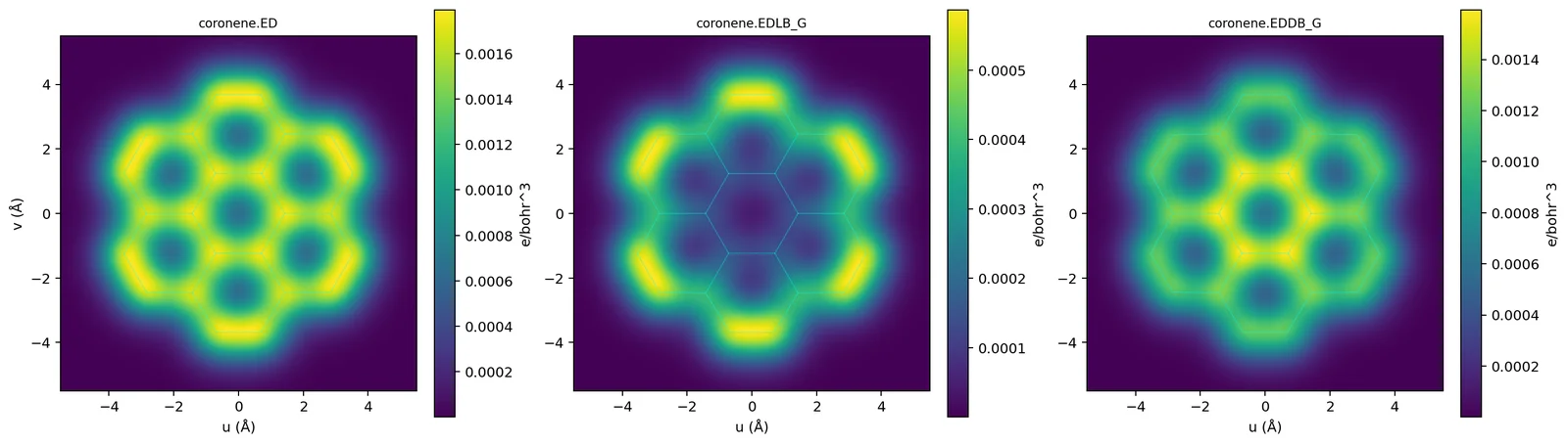
map2png.py draws
the skeleton from coronene.fchk found next to the maps (or from --fchk FILE).| Option | What it sets |
|---|---|
--map-plane fit[,h] | the best-fit plane of the heavy atoms (default), base height h |
--map-plane "ring N[,h]" | the plane of NICS ring N (needs --nics-rings or
--nics-ring) |
--map-plane "atoms i,j,k[,h]" | the plane through three atoms |
--map-plane z=V (or x=, y=) | a plane of the coordinate frame; one plane, no slab (for a section through a molecule) |
--map-slab h1,h2[,n] | average n planes (5) between h1 and h2 Å above the base plane;
none = one plane at the base height |
--map-step H | the lattice step (0.25 Å; 0.05 for figures) |
--cube-margin R | how far the lattice reaches beyond the atoms (10 Å for maps) |
A map file starts with six # lines (the command, the plane origin, normal and in-plane axes,
the lattice, the columns), then one line per node: u v x y z value, the rows of constant u
separated by a blank line. In gnuplot: splot 'mol.EDDB_G.map.dat' using 1:2:6 with pm3d; in
Python: numpy.loadtxt. The plane origin is always a node.
map2png.py options: several files give one row of panels; --clip R shows
|u|, |v| ≤ R; --range A or --range=VMIN,VMAX fixes the colour scale;
--levels 0.01,0.02 adds labelled contour lines; --cmap picks the colour map;
--fchk draws the skeleton.
4. Orbital pictures
Orbitals can be written as cubes, one file per orbital, with an optional list of 1-based indices in brackets:
| Token | Orbitals | Files |
|---|---|---|
nobd[LIST] | natural orbitals for bond delocalization, in the order of --table nobd | mol.NOBD_G_orb001.cube, ... |
no[LIST] | natural orbitals of the density (--table no) | mol.NO_orb001.cube, ... |
ao[LIST] | natural atomic orbitals of the -b basis (--table ao) | mol.NVB_orb001.cube, ... |
bo[LIST] | bond-order orbitals (--table bo) | mol.BO_orb001.cube, ... |
xtb[LIST] | GFN2-xTB molecular orbitals (geometry input) | mol.XTB_orb001.cube, ... |
$ runEDDB -i @benzene -a --export-cube nobd[1-3] --table nobd    # the three pi NOBDs
$ runEDDB -i @benzene -a --export-cube nobd[1-3] --cube-orb2dens # their density, one file
$ runEDDB -i mol.fchk --export-cube ao[2,4,11-15] -b nmb         # selected NMB orbitals
- Lists:
2,4,11-15or both. Without a list every orbital of the lane is written, up to 64 files. --cube-orb2denswrites one file instead, the occupation-weighted density ρ = Σ ni|ψi|2 of the selected orbitals (mol.NOBD_G_density.cube); it integrates to their summed occupation.- Cubes are exact evaluations on the grid and look right in every viewer. Prefer them to FCHK files for pictures of NAOs in large, strongly polarized basis sets.
5. Orbitals for other programs: FCHK and JSON
--export-fchk writes the orbitals as a Gaussian formatted checkpoint file, which GaussView,
Avogadro2, IQmol, Chemcraft and Multiwfn open and which they can turn into cubes themselves.
--export-json writes the same in the ORCA JSON convention.
| Token | FCHK (--export-fchk) | JSON (--export-json) |
|---|---|---|
nobd | NOBDs as MOs, the EDDB density as the total density; mol.NOBD_G.fchk | NOBDs with
their occupations, completed to a square MO matrix; mol.NOBD_G.json |
no | natural orbitals of the density; mol.NO.fchk | the same, real occupations; mol.NO.json |
ao | NAOs of the -b basis; mol.NVB.fchk (NAO / NMB / NVB) | the full NAO set,
independent of -b; mol.NAO.json |
bo | bond-order orbitals of the pairs in the scope; mol.BO.fchk | the same; not orthonormal
between pairs, so read the .json directly; mol.BO.json |
xtb | the GFN2-xTB wavefunction (orbitals, density, spin density); mol.XTB.fchk | the same with
orbital energies; mol.XTB.json |
$ runEDDB -i @benzene -a --export-fchk nobd,no,ao,bo,xtb --export-json xtb --out-dir files
$ ls files
benzene.BO.fchk  benzene.NOBD_G.fchk  benzene.NO.fchk  benzene.NVB.fchk  benzene.XTB.fchk
benzene.XTB.json  benzene.XTB.meta.json
- The index of an orbital in the file equals its row index in the matching table (
--table nobd,no,ao,bo), so the table is the key to the file. - FCHK files store the occupation of each orbital in the orbital-energy field. Avogadro2 shows it as “2.00 eV” for a doubly occupied orbital; viewers that read hartree (GaussView, IQmol, Chemcraft) show the value divided by 27.2114.
- The GFN2-xTB file is a minimal valence basis with an effective core: good as an SCF starting guess for a DFT job or for viewing, not an all-electron result.
- The JSON tokens
ao,no,nobd,boandraweddbneed an ORCA .json input (restricted, spherical, no ECP);xtbneeds a geometry. Every .json comes with a.meta.jsonsidecar describing its contents. --export-json raweddb(diagnostic) writes the matrix from which the EDDB is made, before it is combined with the density: DEDDB = D·R·D. It forces-g -b naoand needs an HF or DFT density. Three square orbital sets store R through its eigenvectors, with the eigenvalues in the Occupancy field:mol.RAWEDDB_bond.json(bonding channel),mol.RAWEDDB_anti.json(anti-bonding channel) andmol.RAWEDDB_sum.json(R = bond + anti). The inter-atomic blocks of the two channels cancel in the sum, so R is block-diagonal over the atoms and its orbitals are one-centre; the bonds reappear only through D·R·D.mol.RAWEDDB_meta.jsonholds the formulas, the atom pairs that passed the bond-order gate and the EDDBG populations. In the AO basis R = C·diag(occ)·CT and DEDDB = D·S·R·S·D.--export-lprojwrites the former projected (compact, polarization-stripped) NAO coefficients to theaoFCHK file, for comparisons with older pictures.
6. Differential maps: comparing two systems
A differential map subtracts a field of a reference system from the same field of a perturbed one,
point by point: Δf = f(this) − f(reference). It shows where a substituent, a hydrogen bond, a
cation above a ring, a solvent or a redox step moves the electrons. There is one token per density:
ded, dedlb, deddb and dbdf. ΔBDFπ
(dbdf under -a) shows the change of the π (de)localization directly in the
language of resonance structures.
The reference is a cube written by an earlier run, given with --cube-ref; it supplies both
the grid and the reference values. Example: benzene and the same ring with Li+ 1.9 Å above
its centre (atoms 1–12 are the benzene in both files):
$ runEDDB -i benzene.xyz    -a -f 1:12 --export-cube bdf --out-prefix ref     # ref.BDF_F.cube
$ runEDDB -i benzene_li.xyz -a -f 1:12 --export-cube dbdf --cube-ref ref.BDF_F.cube
▶ Exporting differential BDF to benzene_li.DBDF_F.cube...                             1s
The result, benzene_li.DBDF_F.cube, is a cube like any other (here it is negative almost
everywhere, between −0.025 and +0.001 e/bohr3). For ΔBDFπ isosurfaces
start around ±0.010.
-a may pick a different number of π NOBDs in the
perturbed system: check --table nobd for both and, if needed, give the same list explicitly with
-s, or the map shows a feature wherever one side lost a contributor. When a clean π
dissection is awkward, deddb and dedlb without -a need no selection and still
show where delocalization is gained or lost.Same frame. A point-by-point difference is only meaningful when both geometries share one
coordinate frame. The safest route is to keep the coordinates of the common fragment fixed in the two
quantum-chemistry jobs. If the frames differ, runEDDB warns (“only 0 of 12 selected atoms overlap the
reference geometry”), and --cube-align fixes it: it superposes the listed atoms on the
reference (Kabsch rotation and translation) and evaluates the field in the reference frame.
$ runEDDB -i benzene_li_rot.xyz -a -f 1:12 --export-cube dbdf --cube-ref ref.BDF_F.cube \
          --cube-align 1:12
    Alignment atoms (--cube-align):    12
    RMSD after rigid alignment:           0.00000 Angstrom
    Max residual displacement:            0.00000 Angstrom
    (arbitrary translation + rotation removed; residual = internal deformation)
Here the complex was rotated and shifted on purpose; the aligned map equals the one above to the
printed precision of the cube. --cube-align removes only a rigid motion. A genuine deformation
of the fragment remains and shows up as the RMSD and the largest residual displacement: when they are
large, the two systems are no longer a small perturbation of each other and the difference map loses its
meaning. The alignment atoms must have the same numbers and elements in both files; without a list
--cube-align uses the -f atoms. It also aligns the orbital cubes of the same run.
In a large molecule that changes shape away from the site you study, restrict both runs to the conserved
region with -f or -p: the densities, the grid and the overlap check then involve only
those atoms.
7. Grid and box
| Option | Effect |
|---|---|
-c N (100) | about N3 points covering the atoms of the scope |
-c -N | about N3 points covering the whole molecule, also under -f /
-p / -r (to show a scoped density in the context of the molecule) |
-c 0 | no cubes at all (the FCHK, JSON and map files are still written; handy in a batch script) |
--cube-margin R (3.2 Å) | the margin added around the atoms on every side |
--cube-ref FILE | copy the grid of an existing cube exactly, so that the new cubes can be added or subtracted point by point in any program |
For the naphthalene ring -p 1-2-3-4-9-10-1 the default grid has a 0.15 bohr step over the ring
atoms; -c -60 gives a 0.31 bohr step over the whole molecule. The magnetic maps have their own
defaults (ICSS 0.5 Å, currents 0.20 Å; see NMR & currents).
8. File names and other files
Every file is named <stem>.<TOKEN>_<SCOPE>.<ext>. The stem is the input
name (@naphthalene gives naphthalene); the scope letter G, H, F, P or R is part of the name
of the scope-dependent fields (EDLB, EDDB, BDF, NOBD and the differentials) and absent from the others (ED, NO,
NAO, XTB). The π dissection changes the contents, not the name.
| Option | Effect |
|---|---|
--out-prefix NAME | replace the stem for every file of the run |
--out-dir DIR | write every file into DIR (created if needed) |
Two runs that differ in scope never overwrite each other; two runs that differ in the dissection do, so give them different prefixes. Other files the program writes:
| File | Written by | Contents |
|---|---|---|
mol.rings | -r | the rings found, one -p string per line
(EDDB analysis) |
mol.nmrref | --table nmr | a shielding reference for chemical shifts (NMR) |
mol.bib, mol.refs.txt | --cite bib|txt|both | the papers to cite for exactly this run |
mol.NMR_DIAG.txt | NMR runs with -v | wide diagnostic tables of the NMR lanes |
mol.NBA_DIAG.csv, mol.NBA_MODES.csv | --table bo -v | the complete balance of every bond order |
9. Viewing the files
- Cubes: VMD, Avogadro2, IQmol, GaussView, Chemcraft, ParaView, Multiwfn. Use a symmetric pair of isosurfaces (±) for BDF, differences and orbitals.
- Map files:
map2png.py(numpy + matplotlib), gnuplot, or any program that reads columns. - FCHK: GaussView, Avogadro2, IQmol, Chemcraft, Multiwfn; the viewer computes the orbital surfaces.
- JSON: ORCA's
orca_2jsonturns the square ones (NO, NOBD, NAO) back into a .gbw file, e.g. as a guess or fororca_plot. - Current density (
.vtk): ParaView, or the scripts described on the NMR page.
Old commands: the removed --output-* options
The one-option-per-file family of the first releases was replaced by the three export verbs:
| Old | New |
|---|---|
-o, --output | --export-cube eddb --export-fchk nobd |
--output-ed, -eddb, -edlb, -bdf | --export-cube ed, eddb,
edlb, bdf (in one list: --export-cube eddb,edlb,bdf) |
--output-ded REF [OUT] (and deddb, dedlb, dbdf) | --export-cube ded --cube-ref REF [--out-prefix OUT] |
--output-nobd, -no, -ao | --export-fchk nobd, no, ao |
--output-xtb [FILE] | --export-fchk xtb [--out-prefix FILE] |
--cube-size 0 FILE | --cube-ref FILE |
10. Methods and references
| Method | Reference |
|---|---|
EDDB / EDLB partition (eddb, edlb) | D.W. Szczepanik, Comput. Theor. Chem. 1080 (2016) 33, doi:10.1016/j.comptc.2016.02.003 |
Bond-delocalization field (bdf, dbdf) | D.W. Szczepanik, P.A. Wieczorkiewicz, ACS Phys. Chem. Au (2026), doi:10.1021/acsphyschemau.6c00031 |
NOBDs (nobd) | D.W. Szczepanik et al., Phys. Chem. Chem. Phys. 16 (2014) 20514, doi:10.1039/c4cp02932a |
Natural atomic orbitals (ao) | A.E. Reed, R.B. Weinstock, F. Weinhold, J. Chem. Phys. 83 (1985) 735, doi:10.1063/1.449486 |
Rigid superposition (--cube-align) | W. Kabsch, Acta Cryst. A32 (1976) 922, doi:10.1107/S0567739476001873 |
GFN2-xTB (xtb) | C. Bannwarth, S. Ehlert, S. Grimme, J. Chem. Theory Comput. 15 (2019) 1652, doi:10.1021/acs.jctc.8b01176 |
ORCA and its JSON format (--export-json) | F. Neese, WIREs Comput. Mol. Sci. 12 (2022) e1606, doi:10.1002/wcms.1606 |