
Szczepanik Research Group
Department of Theoretical Chemistry
Faculty of Chemistry, Jagiellonian University
Gronostajowa 2, 30-387 Krakow, Poland
Tel: (+48) 12 686 23 90
E-mail: dariusz.szczepanik@uj.edu.pl
HOME PROJECTS PUBLICATIONS runEDDB X
About EDDB Download Tutorials Manual
Manual (2026-Nov-03)
High-resolution nc-AFM with a CO-terminated tip shows the bonds of a molecule, and the brightness of a bond follows its bond order. runEDDB computes such images from the electron density with a simple, well-tested model, and splits every image into the share of the localized (EDLB) and the delocalized (EDDB) electrons. The same machinery gives constant-height STM images of the orbitals in a bias window. Both come as 2D maps and as one number per bond.
1. What do you want to see?
| You want | Run |
|---|---|
| an nc-AFM image and its EDLB / EDDB shares | runEDDB -i mol.fchk --export-map afm,afm-edlb,afm-eddb |
| the AFM brightness of every bond, next to its length and bond order | runEDDB -i mol.fchk --table afm |
| the same with the tip closer to the molecule | runEDDB -i mol.fchk --table afm --map-plane fit,3.0 |
| a fullerene or another cage | runEDDB -i c60.fchk --table afm --map-plane radial |
| an STM image of the occupied orbitals within 2 eV of the HOMO | runEDDB -i mol.fchk --export-map stm,stm-edlb,stm-eddb |
| an STM image of the empty orbitals (LUMO side) | runEDDB -i mol.fchk --export-map stm --stm-bias 2 |
| a first look from a geometry alone | runEDDB -i @coronene --table afm --map-plane fit,2.5 |
The coronene examples below use a B3LYP/def2-TZVPP single point (coronene.fchk); each run takes
2–3 s on 16 cores. runEDDB --examples afm lists more, runEDDB --help afm every option.
2. The nc-AFM image
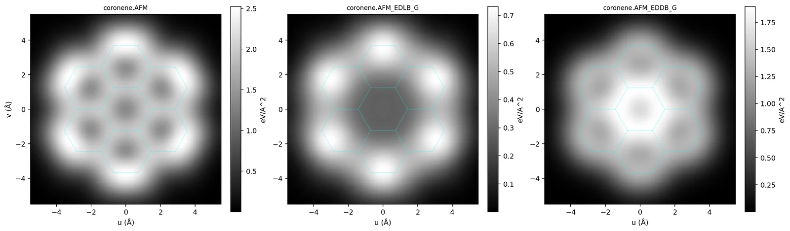
At the small tip heights of bond-resolved imaging the frequency shift is dominated by the Pauli repulsion between the tip and the sample electrons. runEDDB uses the model of Moll et al.: the repulsion is a power of the sample density, V = Aρα (A = 692 eV, α = 0.78 with ρ in e/Å3, their fit for a CO tip), and the image is its curvature ∂2V/∂z2 in eV/Å2, which the frequency shift is proportional to. The tip scans one plane, by default 3.5 Å above the best-fit plane of the heavy atoms.
The image splits into the shares of the localized and the delocalized electrons, VX = VρX/ρ, which add up to the total at every point. The remainder, total − EDLB − EDDB, belongs to the core and Rydberg density outside the analysis block; as a curvature it can have either sign.
$ runEDDB -i coronene.fchk --export-map afm,afm-edlb,afm-eddb --map-step 0.05 --cube-margin 2
$ python3 ~/runEDDB/scripts/map2png.py coronene.AFM.map.dat coronene.AFM_EDLB_G.map.dat \
          coronene.AFM_EDDB_G.map.dat --clip 5.5
3. The contrast of every bond
--table afm prints the image value above the midpoint of every bond with a Wiberg bond order of at
least 0.3, next to its length and bond order: the per-bond form of the bond-order discrimination of Gross
et al. The four C–C bond classes of coronene:
$ runEDDB -i coronene.fchk --table afm
     Bond            R (A)        WBO       total      EDLB_G      EDDB_G
   ───────────   ─────────── ─────────── ═══════════ ─────────── ───────────
     1 C  -  2 C     1.37223     0.78971     2.51580     0.72721     1.34274
     1 C  - 18 C     1.42413     0.62802     2.07798     0.57653     1.32444
     3 C  - 20 C     1.42147     0.63496     1.94154     0.40824     1.61112
    19 C  - 20 C     1.42751     0.61849     1.91103     0.29241     1.87243
tip one plane, h = 3.50 A; V = A rho^0.780, A = 692.0 eV (Moll 2012)| Bond class | total | EDLB share | EDDB share |
|---|---|---|---|
| outer rim, C1–C2 (1.372 Å) | 2.52 | 0.73 | 1.34 |
| rim to the quaternary carbon, C1–C18 | 2.08 | 0.58 | 1.32 |
| spoke, C3–C20 | 1.94 | 0.41 | 1.61 |
| central ring, C19–C20 | 1.91 | 0.29 | 1.87 |
The brightness falls from the short rim bond to the central ring, as the bond order does. In coronene the
difference between the classes is drawn by the localized share (0.73 → 0.29), while the delocalized share
grows in the opposite direction, towards the aromatic core: knowing the density, the delocalization is what the
AFM image does not emphasise. Which share carries the contrast depends on the molecule (in
benzo[k]fluoranthene and hexabenzocoronene it is mainly the EDDB share), so check it with the table for every
system before drawing conclusions. The table also lists the C–H bonds; under -a or -s
the shares are those of the selected NOBDs.
Validation against the bond-order contrast of Gross et al.
On naphthalene, anthracene, phenanthrene, pyrene, triphenylene, coronene, hexa-peri-hexabenzocoronene and
C60 (B3LYP/def2-TZVPP, validation of 2026-09-20) the per-bond contrast correlates with the Wiberg bond
order at r = 0.94–0.98 and with the Pauling bond order from the bond length at r = 0.74–0.96. In
hexabenzocoronene the five C–C classes are ordered monotonically from the peripheral benzo bonds (1.387 Å,
brightest) to the inter-ring bonds (1.461 Å), ratio 1.31; in C60 the 6:6 bonds are brighter than the
6:5 bonds by a factor 1.20 (--map-plane radial).
4. Tip height and model parameters
| Option | Effect |
|---|---|
--map-plane fit,h | tip height h above the best-fit plane (3.5 Å; the atomic-resolution window of Moll et al. is 3.0–4.5 Å). A closer tip sharpens the image and increases the values. |
--map-plane "ring N,h", "atoms i,j,k,h" | the plane of a NICS ring or of three atoms |
--map-plane radial[,h] | for cages: every bond gets its own outward normal from the centre of the
molecule (--table afm, --table stm) |
--map-slab h1,h2[,n] | average n planes between h1 and h2 instead of one plane (the AFM and STM images use one plane by default) |
--map-step, --cube-margin | lattice step (0.25 Å) and how far the lattice reaches beyond the atoms |
--afm-prefactor A, --afm-alpha B | the parameters of V = AρB (692 eV, 0.78), e.g. for another tip |
--afm-tip SIGMA[,s|pz] | research variant: V integrated over a Gaussian tip orbital of width SIGMA (Å), s or pz. The fitted A and α already contain the CO tip, so this is for exploring the tip dependence of the contrast, not a better default. |
5. STM images
For an s-wave tip the tunnelling current at the tip position is proportional to the local density of the sample states between the Fermi level and the bias (Tersoff–Hamann). For a free molecule this is the density of the molecular orbitals inside a bias window, with the HOMO–LUMO gap as the zero of the scale:
--stm-bias Vwith V < 0 (default −2.0) images the occupied MOs from the HOMO down to HOMO − |V| eV; the image splits into EDLB and EDDB shares that add up to the total and integrate to the--table mosums over the window.- V > 0 images the empty MOs from the LUMO up to LUMO + V eV. Virtual orbitals carry no bonding partition, so
only the total map (
--export-map stm) is available. - The values are densities in e/bohr3 at the tip height (3.5 Å), directly comparable with the AFM
image of the same run.
--table stmgives them per bond (10−6 e/bohr3) and states the window in its legend.
$ runEDDB -i coronene.fchk --export-map stm,stm-edlb,stm-eddb --table stm --map-step 0.05 --cube-margin 2
  bias -2.00 V; 6 occupied MOs, eps -7.75 .. -5.75 eV (HOMO)
$ runEDDB -i coronene.fchk --export-map stm --stm-bias 2 --out-prefix cor_p2 --map-step 0.05 --cube-margin 2
$ python3 ~/runEDDB/scripts/map2png.py coronene.STM.map.dat coronene.STM_EDLB_G.map.dat \
          coronene.STM_EDDB_G.map.dat cor_p2.STM.map.dat --clip 5.5 --fchk coronene.fchk
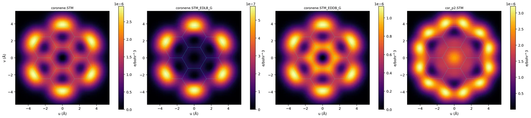
Sweeping the bias reads the orbital spectrum down from the frontier. In coronene the per-bond STM density correlates with the AFM contrast at r = 0.88 at −0.5 V (the HOMO pair only), and at 0.98 at −2 V (6 MOs) and −5 V (18 MOs). In molecules whose frontier orbitals paint a different pattern (benzo[k]fluoranthene) the agreement appears only at a much deeper window.
6. Which wavefunction
- AFM works with every input that gives a density. The model probes the density tail 3–4 Å above the molecule, so use an all-electron HF or DFT wavefunction in a triple-zeta basis or better.
- The GFN2-xTB lane has a minimal basis without that tail: the coronene image is two orders of magnitude
weaker (0.024 instead of 2.5 eV/Å2 for the rim bond). For a qualitative look from a geometry lower the
tip (
--map-plane fit,2.5) and compare contrasts, not values. - STM needs an SCF (HF/DFT) wavefunction with MO coefficients and energies: FCHK, ORCA JSON, Molden, GAMESS, Turbomole. Not the NBO .49 lane, not post-HF densities, not the GFN2-xTB lane.
7. What the model leaves out
Both images are those of the free molecule with a rigid tip. The model has no van der Waals or electrostatic background, no relaxation of the CO tip and no substrate, so it reproduces the contrast within a molecule and not absolute frequency shifts or currents. The apparent shortening of high-order bonds in experimental images comes from the tilting of the CO tip and is outside the model.
8. Methods and references
| Method | Reference |
|---|---|
| High-resolution nc-AFM with a CO tip | L. Gross, F. Mohn, N. Moll, P. Liljeroth, G. Meyer, Science 325 (2009) 1110, doi:10.1126/science.1176210 |
| Pauli-repulsion model of the image, V = Aρα | N. Moll, L. Gross, F. Mohn, A. Curioni, G. Meyer, New J. Phys. 14 (2012) 083023, doi:10.1088/1367-2630/14/8/083023 |
Bond-order discrimination (--table afm) | L. Gross, F. Mohn, N. Moll, B. Schuler, A. Criado, E. Guitián, D. Peña, A. Gourdon, G. Meyer, Science 337 (2012) 1326, doi:10.1126/science.1225621 |
| STM image, Tersoff–Hamann approximation | J. Tersoff, D.R. Hamann, Phys. Rev. B 31 (1985) 805, doi:10.1103/PhysRevB.31.805 |
| EDDB / EDLB partition | D.W. Szczepanik, Comput. Theor. Chem. 1080 (2016) 33, doi:10.1016/j.comptc.2016.02.003 |