
Szczepanik Research Group
Department of Theoretical Chemistry
Faculty of Chemistry, Jagiellonian University
Gronostajowa 2, 30-387 Krakow, Poland
Tel: (+48) 12 686 23 90
E-mail: dariusz.szczepanik@uj.edu.pl
HOME PROJECTS PUBLICATIONS runEDDB X
About EDDB Download Tutorials Manual
◼ Tutorial 8 — Ring-current maps and ACID: who carries the current?
Tutorial 7 gave the ring current as numbers: NICS, Icyc, bond currents. This tutorial draws the same current as pictures: arrows in a plane, streamlines, and ACID surfaces with the current drawn on them, as in Herges’ AICD program. And it adds one thing AICD cannot do: split the current, point by point, into the part carried by delocalized electrons (EDDB) and the part carried by localized ones (EDLB) — without choosing any orbitals.
Before you start
The induced current density J(r) is the first-order response of the electrons to a magnetic field B along the ring normal n; per unit field it is measured in nA/T/Å2. Seen from the +n side, a diatropic current circulates clockwise (aromatic, shielding inside the ring) and is drawn red; a paratropic one circulates anticlockwise (antiaromatic) and is drawn blue. runEDDB splits the current exactly as it splits the shielding: Jtotal = JEDLB + JEDDB + Jother at every point (NMR & currents page of the Manual).
Two Gaussian 16 jobs, B3LYP/def2-TZVPP with NMR=CSGT IOp(10/33=2), are provided (the route sections are in the .gjf files). The .log file must lie next to the .fchk: it carries the exact NMR response; without it runEDDB falls back to the approximate lane and warns that NMR data are missing.
💾 tutorial8_wavefunctions.zip💾 benzene.xyz💾 pentalene.xyz
The zip (7.6 MB) holds _nmr.fchk, _nmr.log and _nmr.gjf for benzene and pentalene. The pictures are drawn by Python scripts installed with the program in ~/runEDDB/scripts/ (they need numpy and matplotlib; the 3D pictures also need POV-Ray).
Part 1 — Benzene: the current in a plane
- --nics-rings 6 — find the six-membered ring and put the NICS probes on it; --rcs adds its ring current Icyc.
- -a — the π-NOBDs. The tables then report the π-part: the first column is EDLB + EDDB of the π-NOBDs, and everything else (σ, core) goes to other. The 3D file gets an extra field, J_EDDB_sel.
- --export-vtk jcur,acid,divj — the current vector field, the ACID scalar and div J on a 3D grid (benzene_nmr.JCUR.vtk, plus JCUR_atoms.vtk for the skeleton).
- --export-map jcur,jcur-eddb — the same current in a plane 1 Å above the ring (.map.dat files).
The warning concerns the shieldings at the nuclei (a basis-set limit of the CSGT response) and does not affect NICS or the current away from them. The π-ring current is 11.30 nA/T, of which 9.99 is carried by the delocalized π-electrons and 1.31 by the localized ones (without -a the table gives the full current, 11.97 nA/T: the σ-electrons add 0.67).
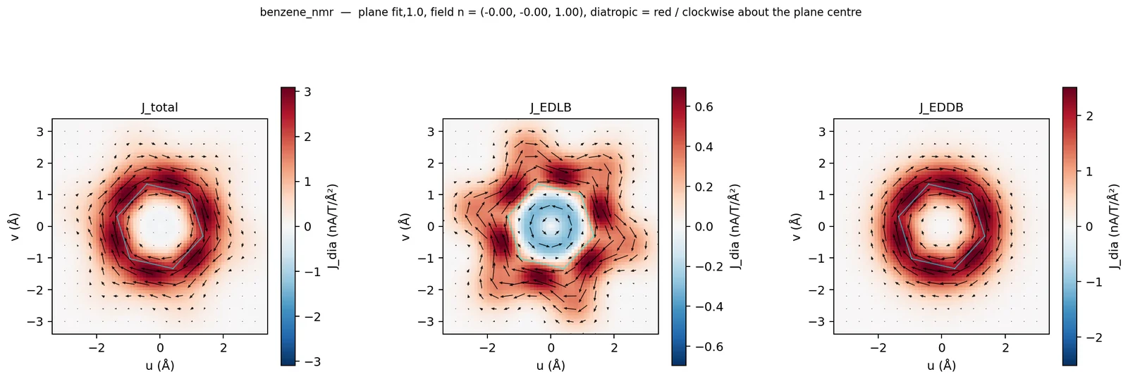
Figure 1. Benzene, plane 1 Å above the ring: Jtotal | JEDLB | JEDDB. Colour = diatropic component (red +, blue −), each panel on its own scale; arrows = in-plane current.
At 1 Å the picture is the familiar diatropic π-torus, and it is JEDDB (maximum about 2.5 nA/T/Å2, right). JEDLB is several times weaker and shows two opposite circulations: diatropic along the C–C and C–H bonds outside, paratropic inside the ring. Add --stream for streamlines:
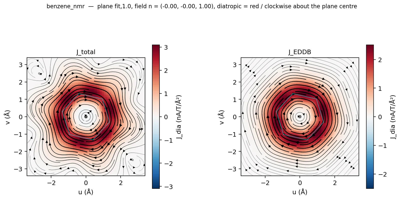
Figure 2. Streamlines of Jtotal and JEDDB, 1 Å above benzene.
In the plane of the ring (--plane fit,0) the σ-electrons dominate. The inner paratropic loop is seen in every picture of the total current, including AICD:
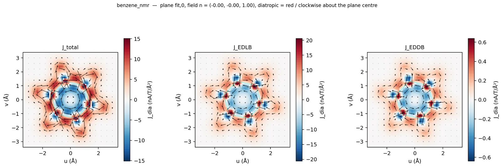
Figure 3. Benzene in the molecular plane: Jtotal | JEDLB | JEDDB.
Part 2 — Benzene in 3D: ACID with the current on it
Each command draws the ACID isosurface of one channel with that channel’s current on it and renders it with POV-Ray. --colour sign colours the arrows red (diatropic) or blue (paratropic); without it they are all green, as in AICD, and the sense is read from the arrows themselves.
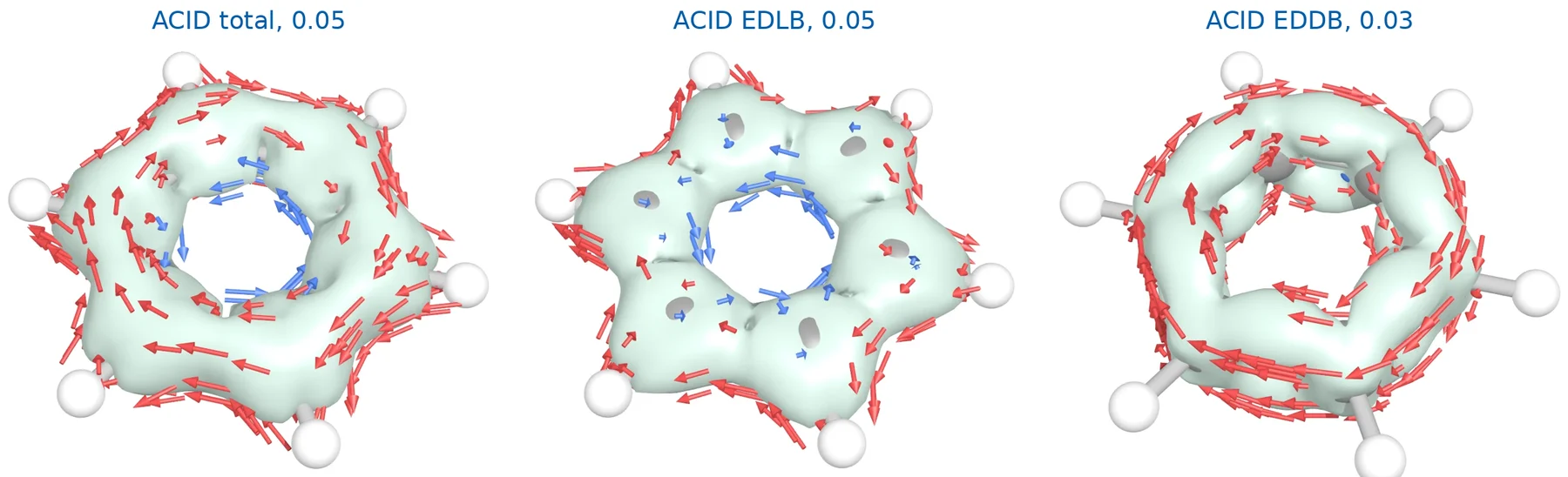
Figure 4. Benzene: ACIDtotal, ACIDEDLB and ACIDEDDB with J on the surface (red = diatropic, blue = paratropic).
Part 3 — Pentalene: a paratropic current carried by localized electrons
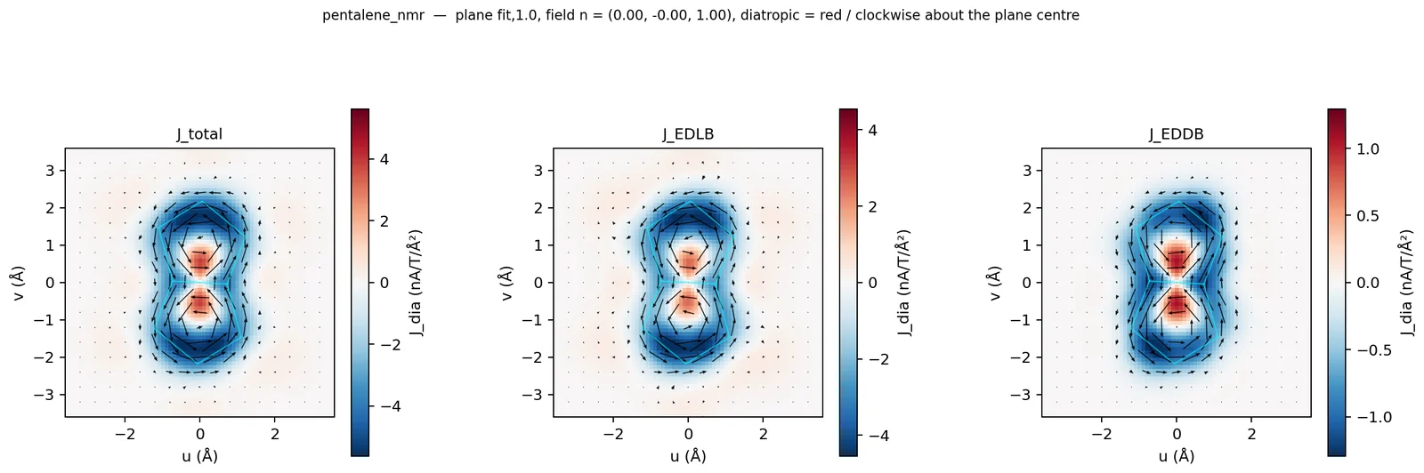
Figure 5. Pentalene (8π, antiaromatic), plane 1 Å above: Jtotal | JEDLB | JEDDB, each on its own scale.
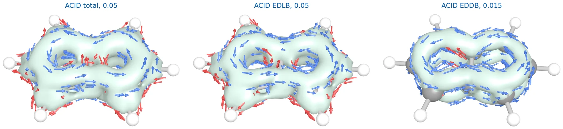
Figure 6. Pentalene: ACIDtotal and ACIDEDLB at 0.05, ACIDEDDB at 0.015 a.u.
Table 1. Benzene and pentalene, B3LYP/def2-TZVPP CSGT, the π-part (-a): π = EDLB + EDDB. Icyc in nA/T, NICS in ppm, populations in e.
| benzene: π | EDLB | EDDB | pentalene (R1 = R2): π | EDLB | EDDB | |
|---|---|---|---|---|---|---|
| Icyc | 11.30 | 1.31 | 9.99 | −21.18 | −15.95 | −5.35 |
| NICS(0) | −19.28 | −2.23 | −17.05 | 13.22 | 10.15 | 3.07 |
| NICS(1)zz | −28.77 | −3.33 | −25.43 | 62.07 | 46.33 | 15.74 |
| π-population | 5.98 | 0.69 | 5.29 | 7.97 | 5.83 | 2.14 |
Part 4 — Should you trust the arrows? The div J table
A current induced by a static field has no sources: div J = 0 everywhere. A finite basis and a finite grid break this a little, and --export-vtk divj measures by how much. The table comes with every 3D export:
- Read the total row: it is the error budget. The largest values are always at the nuclei; the valence columns (r > 0.5 Å from every nucleus) are what the pictures show.
- The valence sources are of the order of the ring current itself (11.2 nA/T for benzene, 21.6 for pentalene), but they are spread over the whole molecule: the ring current read as the flux through a plane agrees with the one integrated along a contour around the ring (11.3 and 11.3 nA/T for benzene). Trust the circulation pattern; do not over-read a single arrow near a nucleus.
- The partial rows add up to more than the total row: the EDLB and EDDB channels exchange current with each other, so each of them alone has sources and sinks. That is a property of the partition, not an error.
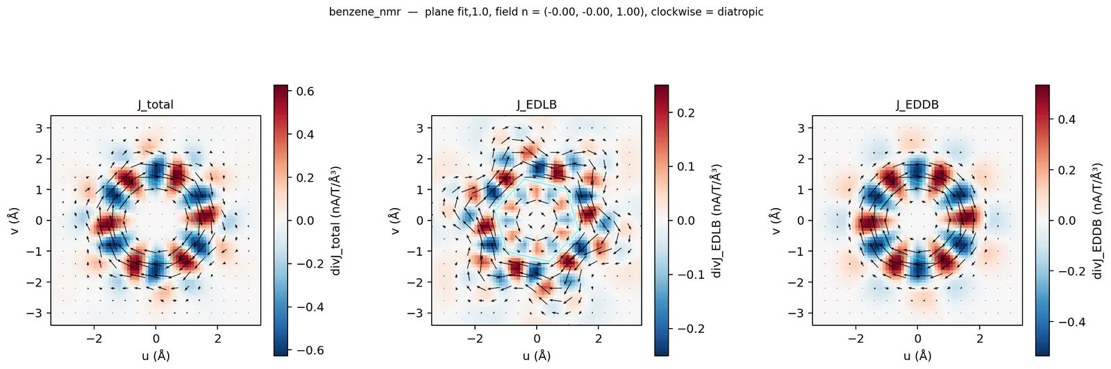
Figure 7. div J of the three channels, 1 Å above benzene.
Part 5 — Without an NMR job
A plain geometry is enough for a qualitative picture. runEDDB then computes the current from its GFN2-xTB orbitals (the APPROXIMATE lane, marked in the stage lines):
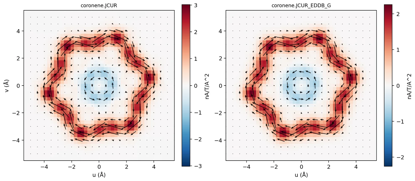
Figure 8. Coronene from a bare geometry (GFN2-xTB, approximate): Jtotal and JEDDB 1 Å above the plane. Diatropic rim, paratropic hub.
The pattern — a diatropic current around the rim and a paratropic one around the hub — is the one known from DFT, and it finishes in half a minute. The magnitudes are not: the uncoupled xTB response is about 40 % too weak (rim Icyc 10.7 nA/T; see the GFN2-xTB page). Use this lane to look, and an NMR job to measure.
Conclusions
- The ring current itself is always read from the flux, Icyc; the pictures tell who carries it.
- In benzene the diatropic π-current is EDDB; the inner paratropic loop is EDLB.
- In pentalene the paratropic current is mostly EDLB: a strong current, few delocalized electrons.
What to try next
- --nmr-mos all,-homo: the current without the HOMO — which orbitals make pentalene paratropic?
- --field-axis for a non-planar molecule or a macrocycle (the Manual describes the cost and the choices).
- Open .JCUR.vtk in ParaView: Contour on ACID_total, Glyph on J_total.
- acid2pov.py --style aicd for the gold-and-green look of the AICD program.