Quick Start — a worked example from start to finish
A good way to get to know runEDDB is to watch it work on a real molecule. This page follows the metallacycle C7H7FeCl from a bare geometry to a reasoned assessment of its aromaticity, introducing along the way the basic, most frequently used options and diagnostics of runEDDB, in context: printing the delocalization summary, requesting specific analysis tables, exporting .cube and .fchk files for visualization, drawing chemical conclusions, and dissecting the π/σ channels — with a word of caution about the automatic --auto-pi screen. It is a primer, not a full reference: many further capabilities (differential density maps, the other scope modes and export targets, and more) live in the Manual — but what you learn here is enough on its own for a basic analysis of systems with delocalized bonds. The whole tutorial runs on runEDDB's built-in GFN2-xTB engine, so you can reproduce every step from nothing but the .xyz file below — no external quantum-chemistry package needed.
⚠ A note on the method. GFN2-xTB is an approximate, semi-empirical tight-binding model — a remarkably good and inexpensive one, more than accurate enough to explore delocalization trends and to drive this tutorial. As a rule it tends to overestimate electron delocalization — but here that is actually a virtue: it lets you first establish whether, for a given ring topology and symmetry, a solution in which the two-center bonds effectively conjugate into a delocalized cycle is possible at all. A subsequent higher-level check — DFT with an exchange–correlation functional that correctly accounts for long-range exchange (a range-separated / long-range-corrected functional such as CAM-B3LYP) — then tests whether exchange–correlation effects preserve that picture or instead drive the system toward bond localization (to avoid excessive same-spin repulsion). Long-range exchange is known to be decisive for a balanced description of electron delocalization and aromaticity (see Szczepanik et al., J. Comput. Chem.38 (2017) 1640; DOI:10.1002/jcc.24805).
1. The molecule and its geometry
This example comes from the original study
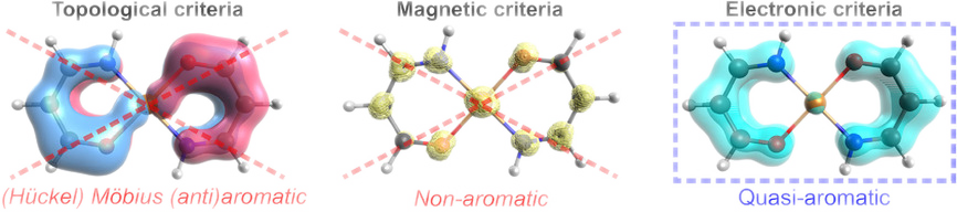
Electron delocalization in planar metallacycles: Hückel or Möbius aromatic?
D.W. Szczepanik (), M. Solà () ChemistryOpen 8 (2019) 219−227. DOI: 10.1002/open.201900014. URL
Abstract:
In this work the relationship between the formal number of π-electrons, d-orbital conjugation topology, π-electron delocalization and aromaticity in d-block metallacycles is investigated in the context of recent findings concerning the correlation of π-HOMO topology and the magnetic aromaticity indices in these species. It is demonstrated that for π-electron rich d-metallacycles the direct link between aromaticity, the number of π-electrons and the frontier π-orbital topology does not strictly hold and for such systems it is very difficult to unambiguously associate their aromaticity with the '4n+2' (Hückel) and '4n' (Möbius) rules. It is also shown that the recently proposed electron density of delocalized bonds (EDDB) method can successfully be used not only to quantify and visualize aromaticity in such difficult cases, but also – in contrast to magnetic aromaticity descriptors – to provide a great deal of information on the real role of d-orbitals in metallacycles without the ambiguity of bookkeeping of electrons in the π-subsystem of the molecular ring. Interestingly, some of the metallacycles studied cannot be classified exclusively as Hückel or Möbius because they have a hybrid Hückel-Möbius or even quasi-aromatic nature.
Everything below starts from a single plain-text geometry file, c7h7fecl.xyz — the 16 atoms of the metallacycle in Cartesian coordinates (Å). Copy the block below into a file, or download it directly:
c7h7fecl.xyz
16

Fe       -0.064251938266      0.000000000000      0.383381287583
C         0.102879051008      1.467437846806     -0.581782848285
C         0.102879051008     -1.467437846806     -0.581782848285
C         0.042058436784      1.945591795572     -1.877580721536
C         0.042058436784     -1.945591795572     -1.877580721535
C        -0.012197738912      1.304915633429     -3.124178523721
C        -0.012197738912     -1.304915633430     -3.124178523721
C        -0.022766917881      0.000000000000     -3.622055704846
H        -0.061079076601      0.000000000000     -4.715595953142
H         0.167516111578      2.281514394810      0.169634195203
H         0.167516111578     -2.281514394810      0.169634195204
H         0.029959638034      3.038668532273     -1.974142731372
H         0.029959638034     -3.038668532273     -1.974142731372
H        -0.055473924074      2.032073158396     -3.942519373400
H        -0.055473924074     -2.032073158396     -3.942519373400
Cl        1.502523783826      0.000000000000      1.822684376427
The atom order fixes the numbering used throughout: atom 1 is Fe, atom 16 is Cl, and atoms 2–8 are the seven carbons of the C7 ring — the labels you will feed to the ring --pathway in Section 4. runEDDB needs no wavefunction for this file: its built-in GFN2-xTB engine builds the one-electron density on the fly, as the next section shows.
2. Global delocalization pattern
First, we investigate the distribution of the electron density of all delocalized bonds in the entire molecule using the EDDBG function (the subscript G stands for global: all atoms and bonds are included). When the input is a geometry rather than a wavefunction, runEDDB automatically builds the one-electron density with GFN2-xTB before running the analysis:
terminal
$ runEDDB --input c7h7fecl.xyz --quiet
The --quiet (or -q) option enables quiet mode: only the EDDBG summary populations are printed — useful for batch jobs where only the numerical result is needed:
output
▶ Printing summary of EDDB calculations:

        Total   ED_G population:           49.82313    per atom:     3.11395
        Total EDLB_G population:           40.56201    per atom:     2.53513
        Total EDDB_G population:            9.26112    per atom:     0.57882

▶ Calculation completed on 2026-07-27. Total time: 0s.
The default analysis basis is the Natural Valence Basis (NVB), which retains only the valence-shell Natural Atomic Orbitals (NAO). GFN2-xTB describes only the valence electrons (a 42-electron effective core potential removes the Fe/Cl/C cores), so of the ~49.8 valence electrons in the NVB about 40.6e are localized (lone pairs and two-center bonds) and ~9.3e are shared through the system of delocalized bonds.
To quickly visualize the EDDBG-layer of the one-electron density, add the --export-cube eddb option:
▶ Exporting EDDB_G to c7h7fecl.EDDB_G.cube...                                         1s
▶ Printing summary of EDDB calculations:

        Total   ED_G population:           49.82313    per atom:     3.11395
        Total EDLB_G population:           40.56201    per atom:     2.53513
        Total EDDB_G population:            9.26112    per atom:     0.57882

▶ Calculation completed on 2026-07-27. Total time: 1s.
This generates a Gaussian cube file (c7h7fecl.EDDB_G.cube) for visualization in, e.g., Avogadro2, IQmol, GaussView, VMD, or Chemcraft; a typical isosurface value is 0.015-0.020. The --ncores (or -n) option parallelizes the grid evaluation, which is the most compute-intensive step; the grid quality is controlled by --cube-size (or -c, default: 100).
To visualize the generated cube file in Avogadro2, select in the program menu Analyze → Create Surfaces and set the parameters as in the figure below:
3. Detailed population analysis
Now, switch to verbose mode with the --verbose (or -v) option. In the current version the analysis tables are opt-in: request them explicitly with --table (here nobd,ao,npa):
First, the program reports what was parsed from the input file:
output
▶ Loading and parsing input file...                                                   0s

    Source file:                       c7h7fecl.xyz
    File format:                       XYZ geometry
    Structures in file:                1
    Number of atoms:                   16
    Center input geometry:             No
    Charge / multiplicity:             0 / 1
Because the input is a plain geometry, runEDDB models the one-electron density itself with its built-in GFN2-xTB engine (semi-empirical tight-binding with DFT-D4 dispersion) in a minimal Slater-type vSTO-nG basis. A 42-electron effective core potential leaves 50 valence electrons in 53 basis functions, and the SCC converges in a handful of iterations:
output
▶ Modelling one-electron density at the GFN2-xTB/vSTO-nG level...

    Hamiltonian model:                 GFN2-xTB
    Dispersion correction:             DFT-D4
    Initial guess:                     SAD
    Algorithm:                         SCC
    Maximum SCC iterations (MAXITER):  1500
    Convergence criterion (CONV):      1.00E-04 (max|dq|)
    Anisotropic electrostatics (AES):  Enabled
    Spin polarization (SP):            Disabled
    Fermi smearing (ETEMP):            Enabled (300 K)
    Effective core potential:          Yes (42 core electrons)
    Number of basis functions:         53 (vSTO-nG)
    Total energy:                      -26.08073 Eh  (18 SCC iterations)
    Electron population (Tr[D*S]):     50.00000
    SCC time:                          0s
    Papers to be cited (DOI):          10.1021/acs.jctc.8b01176 (GFN2-xTB)
                                       10.1063/1.5090222 (DFT-D4)
Next, it summarises the internal AO→NAO localization procedure:
output
▶ Building natural atomic orbitals (NAO, frozen-NMB two-cycle)...                     0s

    NAO algorithm:                     Frozen-NMB (two-cycle construction)
    Total number of NAOs:              53 = 0 (Cor) + 45 (Val) + 8 (Ryd)
    Total electron population:         50.00000
            - core population:         0.00000 (~0.0 %)
         - valence population:         49.82313 (~99.6 %)
         - rydberg population:         0.17687 (~0.4 %)
    Target NAO representation:         Natural valence basis (NVB = Val)
             - NVB population:         49.82313 (~99.6 %)
    Papers to be cited (DOI):          10.1063/1.449486 (NAO)
                                       in preparation (frozen-NMB)
Out of the 53 NAOs, none are core (the ECP already removed them), 45 are valence (Val) and 8 are Rydberg (Ryd). The default NAO representation (NVB) keeps only the 45 valence NAOs that capture ~49.8e — the analysis below operates on this subspace.
In the next stage the program prints the BOP configuration and performs the calculations:
output
▶ Performing multicenter bond-orbital projections (BOP)...

    Type of EDDB function:             EDDB_G (entire molecular system)
    BOP algorithm:                     Standard BOP (HF/DFT 1-densities)
    Atoms included in BOP:             16
    Pairs included in BOP:             62
    Bond-order threshold:              0.00100
    Connectivity mask basis:           full NAO
    Number of BOP cycles:              1
    BOP time:                          0.007s
    Papers to be cited (DOI):          10.1016/j.cplett.2014.01.006 (BOP)
                                       10.1016/j.comptc.2016.02.003 (EDDB)
                                       10.1002/open.201900014 (EDDB-AO)
In the entire system, 62 atom pairs exceed the Wiberg bond-order threshold (10−3) and enter the BOP cycle.
After the BOP step, the program prints the requested electron-population tables. The first lists the Natural Orbitals for Bond Delocalization (NOBD):
The table shows that the first five NOBDs make the dominant contributions to electron delocalization. Their orbital decomposition reveals that the first three NOBDs have almost purely π-symmetry (~1.6-1.8e, 99-100% p-character), while the fourth and fifth involve the Fe atom through its 3d orbitals (~63% and ~88% d-character, respectively). The remaining NOBDs have much smaller occupancies associated with σ-delocalization tails.
The next table presents the population analysis in atomic-orbital resolution — one row per NAO in the target representation (here NVB, valence-only). It reports both the total electron population (EDG) and the delocalized component (EDDBG) per orbital:
The data reveal that the main delocalization channels involve the 3d orbitals on Fe (the 3d5 and 3d2 components contribute ~0.84e and ~0.45e to delocalization) together with the 2p1 orbitals on the carbon atoms (~0.7-0.9e each). Electrons on chlorine and hydrogen atoms are predominantly localized.
Finally, the last table collapses the data to condensed-atomic resolution, adding the natural atomic charge (qN) of each atom:
output
  ┌────────────────────────────────────────────────────────────────────────────────────┐
  │          NATURAL POPULATION ANALYSIS IN CONDENSED-ATOMIC (NVB) RESOLUTION          │
  └────────────────────────────────────────────────────────────────────────────────────┘
     Atom      Charge       ED_G        α         β        EDDB_G       α         β
   ────────   ─────────   ───────── ───────── ─────────   ═════════ ───────── ─────────
       1 Fe   +1.22153     6.60631      -         -        1.75000      -         -
       2 C    -0.31665     4.31665      -         -        1.07054      -         -
       3 C    -0.31665     4.31665      -         -        1.07054      -         -
       4 C    -0.02589     4.02589      -         -        0.98681      -         -
       5 C    -0.02589     4.02589      -         -        0.98681      -         -
       6 C    +0.01454     3.98546      -         -        0.89438      -         -
       7 C    +0.01454     3.98546      -         -        0.89438      -         -
       8 C    -0.03227     4.03227      -         -        0.97527      -         -
       9 H    +0.01810     0.98190      -         -        0.02363      -         -
      10 H    -0.00186     1.00186      -         -        0.04202      -         -
      11 H    -0.00186     1.00186      -         -        0.04202      -         -
      12 H    +0.02389     0.97611      -         -        0.04584      -         -
      13 H    +0.02389     0.97611      -         -        0.04584      -         -
      14 H    +0.01783     0.98217      -         -        0.02017      -         -
      15 H    +0.01783     0.98217      -         -        0.02017      -         -
      16 Cl   -0.63108     7.62637      -         -        0.39271      -         -
   ────────   ─────────   ───────── ───────── ─────────   ═════════ ───────── ─────────
The numbers confirm that only Fe and the ring C atoms contribute significantly to the global delocalization, while the Fe center carries a sizeable positive charge (~+1.2) and the Cα atoms (2, 3) are the most negative (~−0.32). A condensed-atomic table like this one is the starting point for most discussions and is sufficient for many quick assessments.
4. Cyclic delocalization of π-electrons
Aromatic stabilization in molecular rings with π-conjugated bonds is associated with cyclic delocalization of π-electrons, whereas cross-ring orbital interactions are often locally destabilizing (cf. the antibonding interaction between para-related carbon atoms in benzene). To assess the effect of cyclic π-electron delocalization in the 8-membered ring (8MR) of the C7H7FeCl system, we perform an EDDBP calculation (the subscript P stands for pathway):
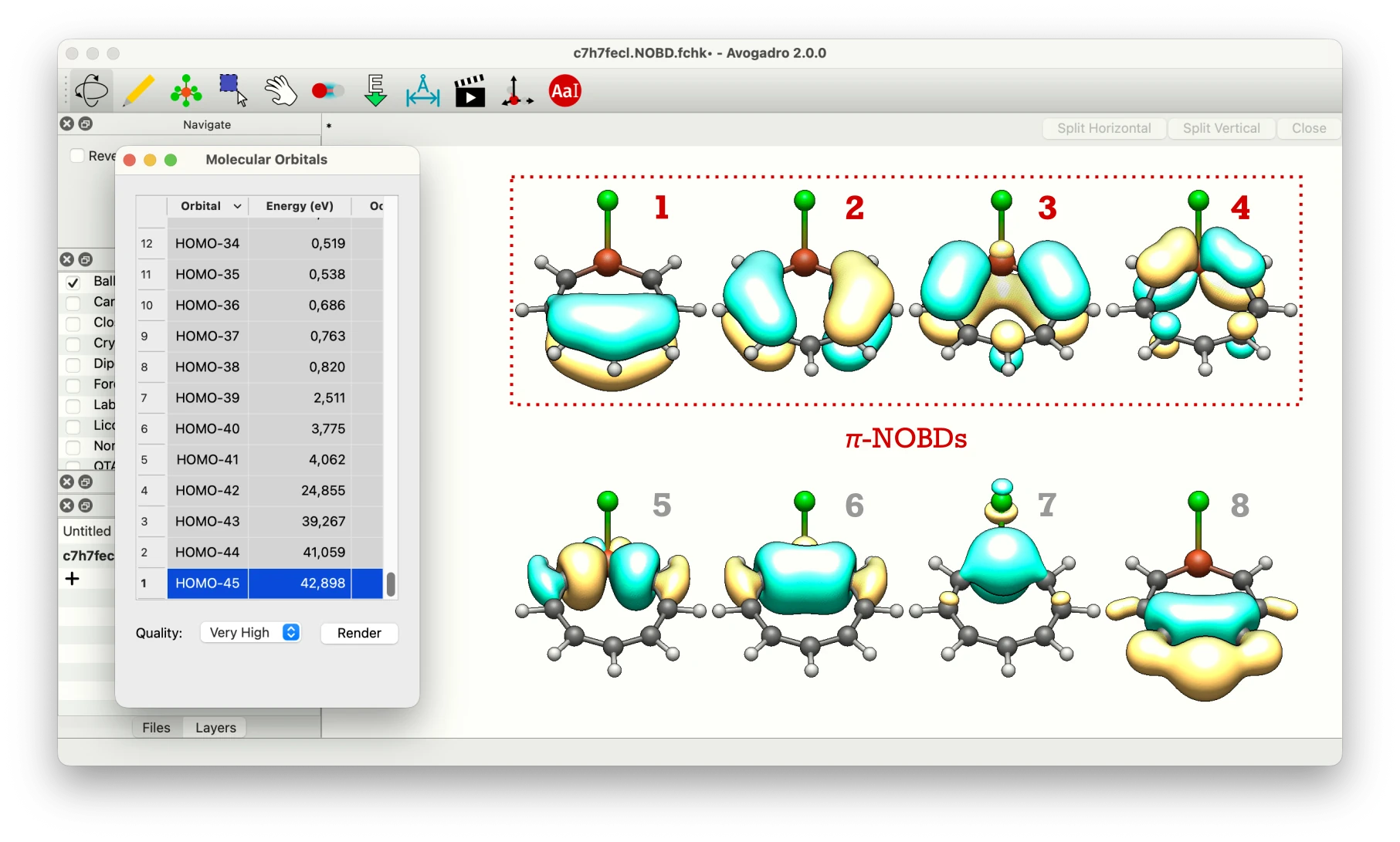
The --pathway (or -p) option specifies the bond connectivity along the ring. The --export-fchk nobd option generates a new Gaussian FCHK file (c7h7fecl.NOBD_P.fchk) in which the Alpha MO coefficients are replaced by the spinless NOBDs. The --auto-pi (or -a) option automatically selects only π-type NOBDs based on their orbital composition (marked with * in the Sel column):
The --auto-pi option identifies the first five NOBDs as π-orbitals; together they account for ~9.9e of π-electrons, of which ~5.97e is cyclically delocalized. To visually inspect the NOBDs and verify the automatic π-NOBD selection, open the generated c7h7fecl.NOBD_P.fchk file in Avogadro2 and select a particular NOBD in the Molecular Orbitals window (in the generated file the α-MOs ordered by increasing energy are replaced by NOBDs ordered by decreasing occupation number):
As follows from the summary, the average per-atom population of cyclically delocalized π-electrons in the 8MR is 0.74610e. However, the EDDBP atomic populations reveal that the distribution is not uniform: a noticeable π-deficiency on atoms 2 and 3 (~0.635e vs ~0.78e on atom 8) is a fingerprint of high-energy ionic resonance structures contributing to the wavefunction and reducing the aromatic stabilization energy.
A word of caution: --auto-pi is a fast automatic screen based on orbital composition, not the last word. Here it is worth a second look — the fifth selected NOBD is only weakly occupied (~0.35e) and heavily d-type (~88% d), so it sits on the borderline between the π- and the σ/d-subsystems. Good practice is to verify the selection visually in the exported c7h7fecl.NOBD_P.fchk and, if desired, override it explicitly with --select-nobd (or -s). Keeping only the four dominant π-NOBDs recovers the textbook 8π picture:
▶ Loading and parsing input file...                                                   0s
▶ Modelling one-electron density at the GFN2-xTB/vSTO-nG level...                     0s
▶ Building natural atomic orbitals (NAO, frozen-NMB two-cycle)...                     0s
▶ Performing multicenter bond-orbital projections (BOP)...                            0s
▶ Computing natural orbitals for bond delocalization (NOBD)...                        0s
▶ Printing analysis details:

  ┌────────────────────────────────────────────────────────────────────────────────────┐
  │          NATURAL POPULATION ANALYSIS IN CONDENSED-ATOMIC (NVB) RESOLUTION          │
  └────────────────────────────────────────────────────────────────────────────────────┘
     Atom      Charge       ED_P        α         β        EDDB_P       α         β
   ────────   ─────────   ───────── ───────── ─────────   ═════════ ───────── ─────────
       1 Fe   +1.22153     1.27643      -         -        0.68154      -         -
       2 C    -0.31665     0.90292      -         -        0.62513      -         -
       3 C    -0.31665     0.90292      -         -        0.62513      -         -
       4 C    -0.02589     0.99708      -         -        0.75349      -         -
       5 C    -0.02589     0.99708      -         -        0.75349      -         -
       6 C    +0.01454     0.95041      -         -        0.70359      -         -
       7 C    +0.01454     0.95041      -         -        0.70359      -         -
       8 C    -0.03227     1.00071      -         -        0.77862      -         -
   ────────   ─────────   ───────── ───────── ─────────   ═════════ ───────── ─────────

▶ Printing summary of EDDB calculations:

        Total   ED_P population:            7.97795    per atom:     0.99724
        Total EDLB_P population:            2.35336    per atom:     0.29417
        Total EDDB_P population:            5.62459    per atom:     0.70307

    Cyclic Delocal. Index (CDI):            0.62513

▶ Calculation completed on 2026-07-27. Total time: 0s.
With exactly four π-NOBDs the ring now carries ~7.98e (the formal 8π count), of which ~5.62e is cyclically delocalized. Dropping the small d-heavy NOBD trims ~2e and lowers the per-atom population only slightly — the physical picture is unchanged, which is reassuring.
The Cyclic Delocalization Index (CDI), printed at the end of the summary, equals the smallest per-atom EDDBP value — the maximum population of π-electrons (per atom) that can be uniformly delocalized around the cycle. Here the CDI is ~0.625 (~0.635 with the automatic five-NOBD selection); for comparison, the CDI of benzene at the same GFN2-xTB level is ~0.889 (run runEDDB -i benzene.xyz -p 1-2-3-4-5-6-1 -a -q to reproduce it), so the relative π-aromaticity in the 8MR of C7H7FeCl can be estimated as ~70%.
5. 3d-orbital conjugation topology
The remaining open question is: what does the dominant Fe 3d orbital look like? To find out, dissect the π-channel in atomic-orbital resolution and export the valence NAOs:
terminal
$ runEDDB --input c7h7fecl.xyz --pathway 1-2-4-6-8-7-5-3-1 --auto-pi --export-fchk ao --table ao
The --export-fchk ao option writes the valence NAOs to c7h7fecl.NVB.fchk. According to the resulting NVB-resolution table,
output
▶ Loading and parsing input file...                                                   0s
▶ Modelling one-electron density at the GFN2-xTB/vSTO-nG level...                     0s
▶ Building natural atomic orbitals (NAO, frozen-NMB two-cycle)...                     0s
▶ Performing multicenter bond-orbital projections (BOP)...                            0s
▶ Computing natural orbitals for bond delocalization (NOBD)...                        0s
▶ Exporting NVB orbitals to c7h7fecl.NVB.fchk...                                      0s
▶ Printing analysis details:

  ┌────────────────────────────────────────────────────────────────────────────────────┐
  │           NATURAL POPULATION ANALYSIS IN ATOMIC-ORBITAL (NVB) RESOLUTION           │
  └────────────────────────────────────────────────────────────────────────────────────┘
    Index   NVB    Atom      ED_P        α         β       EDDB_P       α         β
   ─────── ───── ────────  ───────── ───────── ─────────  ═════════ ───────── ─────────
        1   4s       1 Fe   0.01867      -         -       0.01095      -         -
        2   3d1      1 Fe   0.00939      -         -       0.00182      -         -
        3   3d2      1 Fe   1.33548      -         -       0.23367      -         -
        4   3d3      1 Fe   0.05064      -         -       0.02694      -         -
        5   3d4      1 Fe   0.41971      -         -       0.07668      -         -
        6   3d5      1 Fe   1.20562      -         -       0.63937      -         -
        7   2s       2 C    0.01080      -         -       0.00602      -         -
        8   2p1      2 C    0.92891      -         -       0.61779      -         -
        9   2p2      2 C    0.01466      -         -       0.00908      -         -
       10   2p3      2 C    0.00398      -         -       0.00218      -         -
       11   2s       3 C    0.01080      -         -       0.00602      -         -
       12   2p1      3 C    0.92891      -         -       0.61779      -         -
       13   2p2      3 C    0.01466      -         -       0.00908      -         -
       14   2p3      3 C    0.00398      -         -       0.00218      -         -
       15   2s       4 C    0.00016      -         -       0.00006      -         -
       16   2p1      4 C    1.02618      -         -       0.75641      -         -
       17   2p2      4 C    0.00053      -         -       0.00032      -         -
       18   2p3      4 C    0.00306      -         -       0.00226      -         -
       19   2s       5 C    0.00016      -         -       0.00006      -         -
       20   2p1      5 C    1.02618      -         -       0.75641      -         -
       21   2p2      5 C    0.00053      -         -       0.00032      -         -
       22   2p3      5 C    0.00306      -         -       0.00226      -         -
       23   2s       6 C    0.00004      -         -       0.00003      -         -
       24   2p1      6 C    0.95082      -         -       0.70244      -         -
       25   2p2      6 C    0.00011      -         -       0.00008      -         -
       26   2p3      6 C    0.00210      -         -       0.00151      -         -
       27   2s       7 C    0.00004      -         -       0.00003      -         -
       28   2p1      7 C    0.95082      -         -       0.70244      -         -
       29   2p2      7 C    0.00011      -         -       0.00008      -         -
       30   2p3      7 C    0.00210      -         -       0.00151      -         -
       31   2s       8 C    0.00002      -         -       0.00001      -         -
       32   2p1      8 C    1.02513      -         -       0.78196      -         -
       33   2p2      8 C    0.00001      -         -       0.00001      -         -
       34   2p3      8 C    0.00139      -         -       0.00106      -         -
   ─────── ───── ────────  ───────── ───────── ─────────  ═════════ ───────── ─────────

▶ Printing summary of EDDB calculations:

        Total   ED_P population:            9.94875    per atom:     1.24359
        Total EDLB_P population:            3.97995    per atom:     0.49749
        Total EDDB_P population:            5.96880    per atom:     0.74610

    Cyclic Delocal. Index (CDI):            0.63506

▶ Calculation completed on 2026-07-27. Total time: 0s.
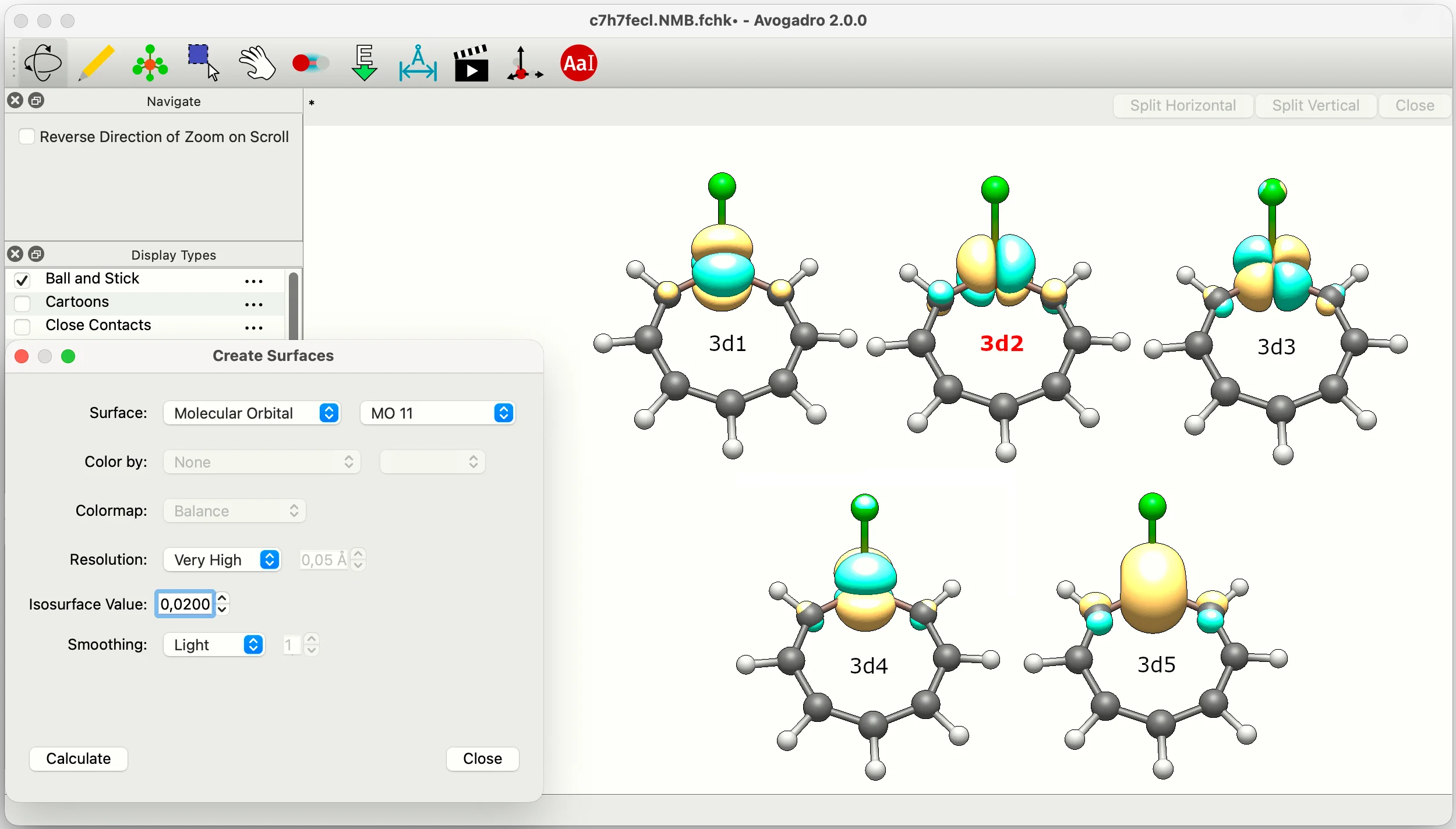
the dominant d-channel is the 3d5 (Fe) orbital — index 6 — carrying ~0.64e of cyclically delocalized π-density (by far the largest Fe contribution). Opening c7h7fecl.NVB.fchk in Avogadro2 (Analyze → Create Surfaces) and inspecting Molecular Orbital no. 6 reveals a 3dXY orbital, which means the metallacycle is a Möbius-Craig aromatic with a predominantly δ-type conjugation topology (see the reference paper for more examples of metallacycles with π- and δ-conjugation topology).
6. Final conclusion
The EDDB analysis at the GFN2-xTB level reveals that the model C7H7FeCl metallacycle (in its ground-state configuration) can be classified as a Möbius-Craig aromatic species with a predominating δ-conjugation topology involving the 3dXY (Fe) orbital. The effectiveness of cyclic delocalization of π-bonds in this 8-membered ring is relatively high — about 70% of the one in the archetypal π-aromatic benzene evaluated at the same level of theory. Bear in mind, however, that this GFN2-xTB result is a fast, first-pass approximation and should be verified with ab initio calculations (long-range-corrected DFT or higher).
7. Preparing ab-initio inputs for quantum-chemistry programs
As the conclusion warns, a GFN2-xTB result is a fast first pass and should be confirmed at an ab-initio level. The reassuring part is that the EDDB analysis itself is identical regardless of the source program — only the way you generate the wavefunction file differs. Below, for each supported package, we show how to run the same C7H7FeCl single-point at the CAM-B3LYP/def2-SVP level (a long-range-corrected functional, important for a balanced description of delocalization) and hand the result to runEDDB with a simple runEDDB --input … call. All example input files are collected in the runEDDB_inputs/ folder; once the wavefunction file exists, every step of the tutorial above is the same for all programs.
▸ Gaussian — input file: 💾 c7h7fecl.gjf. The route section requests the density and a formatted checkpoint (# CAM-B3LYP/def2SVP FormCheck). Run Gaussian G16 (tested: ES64L-G16RevC.01) and rename the resulting Test.FChk, then run the analysis directly on the FCHK file:
terminal
$ g16 c7h7fecl.gjf && mv Test.FChk c7h7fecl.fchk
terminal
$ runEDDB --input c7h7fecl.fchk
▸ Q-Chem — input file: 💾 c7h7fecl.in. The GUI = 2 setting tells Q-Chem (tested: 6.4.0-1) to write a formatted checkpoint (c7h7fecl.fchk). Run the single-point and feed the checkpoint to runEDDB:
terminal
$ qchem -nt 4 c7h7fecl.in >& c7h7fecl.out
terminal
$ runEDDB --input c7h7fecl.fchk
▸ ORCA — input file: 💾 c7h7fecl.inp. After the SCF, convert the binary c7h7fecl.gbw to the JSON wavefunction format with orca_2json (ORCA, tested: 6.0.1); this writes c7h7fecl.json, which runEDDB reads directly:
▸ GAMESS-US — input file: 💾 c7h7fecl.inp. Because GAMESS does not ship the def2 family natively, the basis set is embedded in the input; the job uses ISPHER=1 (spherical harmonics) and DGRID=.T. (high-precision F17.10 MOs, recommended for post-processing). Run the job and analyse the GAMESS output file:
terminal
$ rungms c7h7fecl 00 4 > c7h7fecl.gms
terminal
$ runEDDB --input c7h7fecl.gms
▸ Turbomole — coordinate file: 💾 coord (Cartesian coordinates in Bohr, native Turbomole format). Turbomole has no single input file: place coord in an empty working directory and let the define tool build control, basis and the EHT guess. The whole interactive session can be driven non-interactively by piping the answer sequence on stdin (def2-SVP on all atoms, CAM-B3LYP via libxc, default charge / multiplicity / occupations):
terminal
$ echo -e "\nC7H7FeCl\na coord\n*\nno\nb all def2-SVP\n*\neht\ny\n0\ny\ndft\non\nfunc hyb_gga_xc_cam_b3lyp\n*\n*\n" | define
Then run the SCF with dscf and concatenate control + coord + basis + mos into a single c7h7fecl.tmol bundle that runEDDB reads directly:
terminal
$ dscf && cat control coord basis mos > c7h7fecl.tmol
terminal
$ runEDDB --input c7h7fecl.tmol
8. Command cheat-sheet for C7H7FeCl
Every command used above, in one place — copy, paste, and adapt. Below the tutorial commands, a compact reference to the three things you steer on every run: what to analyse (scope modes), what to report (analysis tables), and what to export for visualization.
runEDDB — every command used above
$ runEDDB -i c7h7fecl.xyz -q # EDDB_G summary only (quiet mode)$ runEDDB -i c7h7fecl.xyz --export-cube eddb -n 4 # global EDDB_G cube for viewing$ runEDDB -i c7h7fecl.xyz -v --table nobd,ao,npa # full population analysis$ runEDDB -i c7h7fecl.xyz -p 1-2-4-6-8-7-5-3-1 -a --export-fchk nobd --table nobd,npa # ring CDI (π, auto)$ runEDDB -i c7h7fecl.xyz -p 1-2-4-6-8-7-5-3-1 -s 1:4 --table npa # override: keep 4 π-NOBDs$ runEDDB -i c7h7fecl.xyz -p 1-2-4-6-8-7-5-3-1 -a --export-fchk ao --table ao # dissect the 3d channel$ runEDDB -i c7h7fecl.fchk # identical analysis on an ab-initio wavefunction
1 · Choose what to analyse — the five scope modes (-g / -h / -f / -p / -r)
One mutually-exclusive flag selects the region of delocalization the analysis (and any exported cube) focuses on. They are the backbone of an EDDB study:
--global / -g — EDDBG: the whole molecule (the default). The global delocalization picture.
--heavy-atoms / -h — EDDBH: the whole molecule like EDDBG, but every connection to a hydrogen is dropped from the connectivity before the analysis. The natural sibling of EDDBG (and the scope recommended as default in the legacy runEDDB.R): faster on large π-conjugated systems, and it keeps C–H hyperconjugation out of the π-NOBD picture (no σ/π mixing). (Note: -h is this scope, not help — use --help.)
--fragment / -f LIST — EDDBF: restrict the populations / cube to a chosen set of atoms, e.g. -f 1:6,10,12 — the rest of the molecule is still fully present in the wavefunction.
--pathway / -p CHAIN — EDDBP: a specific cyclic pathway, e.g. -p 1-2-3-4-5-6-1 (repeat the first atom to close the ring). This is how you get the Cyclic Delocalization Index (CDI) — a direct, quantitative aromaticity measure.
--ring-detect / -r LIST — EDDBR: automatically find every n-membered ring (sizes you ask for, e.g. -r 6 or -r 5,6,7) in the bond-order graph and run a CDI on each — an automatic -p over the whole molecule, with the full ring list written to <stem>.rings.
See §3 Analysis Modes for the full details (plus NOBD dissection and the NAO basis subsets).
2 · Read the bonding — universal analysis tables (--table)
These print straight to the terminal — no file written — and are powerful, universal one-liners that work on any wavefunction the program can read. Two of them stand out:
--table npa — Natural Population Analysis: natural atomic charges qN (ECP- and GFN2-aware), orbital- and condensed-atomic populations, and the per-atom electron delocalization. A complete, NBO-quality population analysis from any input.
--table bo — Bond-Order Orbitals: each pair’s (Wiberg) bond order resolved into orthonormal bond-order orbitals, each carrying a σ/π/δ/φ symmetry label — a spin- and correlation-consistent generalisation of the bond index, the textbook way to see what a bond is made of. (Aliases boo / nba are accepted; add --export-fchk bo to write the orbitals for viewing.)
(--table no adds the natural-orbital occupancy table, with its multireference / spin-contamination indices shown under -v; --table nobd the NOBD-resolution table; --table mo the per-MO ED / EDLB / EDDB decomposition when canonical MOs are present; --table all emits everything.) For example, what a benzene C–C bond is actually made of — one command:
runEDDB -i benzene.fchk --table bo
  ┌────────────────────────────────────────────────────────────────────────────────────┐
  │                       BOND-ORDER ORBITALS (BOO) IN NVB BASIS                       │
  └────────────────────────────────────────────────────────────────────────────────────┘
    Index      Atom pair         Total        BOO occupations with symmetry labels
   ─────── ─────────────────   ─────────  ─────────────────────────────────────────────
        1      1~2      C~C     1.44010    0.97498(σ) 0.44444(π) 0.01997(π) 0.00071(σ)
        5      1~4      C~C     0.11731    0.11111(π) 0.00383(σ) 0.00236(π)
        8      1~6      C~C     1.44010    0.97498(σ) 0.44444(π) 0.01997(π) 0.00071(σ)
       12      1~7      C~H     0.97256    0.97256(σ)
        … (atoms 2–6 repeat the same C–C and C–H pattern)
   ─────── ─────────────────   ─────────  ─────────────────────────────────────────────
    (σ/π/δ/φ = bond-orbital symmetry; Total = full Wiberg index over all BOOs)

  Each row leads with the global Index of the pair’s first BOO (its last is implicit
  — one below the next row’s Index — and matches the MO numbering of --export-fchk bo).
  Each aromatic C–C bond resolves into 0.975 σ + 0.444 π — the π piece is
  exactly the delocalized component EDDB maps; the weak 1–4 "meta" interaction
  is pure π; every C–H is a single σ.
3 · Export for visualization (--export-cube / --export-fchk)
Write Gaussian .cube volumetric fields (ed, eddb, edlb, bdf, their differential maps, and per-orbital cubes via ao|no|nobd|bo|xtb[LIST] — one exactly-evaluated cube per selected orbital, faithful in any viewer) or Gaussian .fchk orbitals (nobd, no, bo, the ao basis set, or the GFN2-xTB wavefunction) for any cube/FCHK viewer. Each verb takes a comma-separated list, so one call can emit many coherent files at once. See §5 Output Files and §6 Differential Maps.
Where to go next. The full reference lives in the Manual: §2 covers every input format and the built-in GFN2-xTB engine; §3 the analysis modes; §4 every command-line option; §5–§7 the outputs and how to read them.