aromaticity.uj.edu.pl

Szczepanik Research Group

Department of Theoretical Chemistry
Faculty of Chemistry, Jagiellonian University
Gronostajowa 2, 30-387 Krakow, Poland
Tel: (+48) 12 686 23 90
E-mail: dariusz.szczepanik@uj.edu.pl

ABOUT US       PROJECTS       PUBLICATIONS       EDDB       TUTORIALS       X

Aromaticity       About EDDB       Installation       Quick start

---

◼Aromaticity

IUPAC definition of aromaticity (Pure Appl. Chem. 1999, 71 , 1919  URL   ):

“The concept of spatial and electronic structure of cyclic molecular systems displaying the effects of cyclic electron delocalization which provide for their enhanced thermodynamic stability (relative to acyclic structural analogues) and tendency to retain the structural type in the course of chemical transformations.

A quantitative assessment of the degree of aromaticity is given by the value of the resonance energy. It may also be evaluated by the energies of relevant isodesmic and homodesmotic reactions. Along with energetic criteria of aromaticity, important and complementary are also a structural criterion (the lesser the alternation of bond lengths in the rings, the greater is the aromaticity of the molecule) and a magnetic criterion (existence of the diamagnetic ring current induced in a conjugated cyclic molecule by an external magnetic field and manifested by an exaltation and anisotropy of magnetic susceptibility).

Although originally introduced for characterization of peculiar properties of cyclic conjugated hydrocarbons and their ions, the concept of aromaticity has been extended to their homoderivatives (see homoaromaticity), conjugated heterocyclic compounds (heteroaromaticity), saturated cyclic compounds (σ) as well as to three-dimensional organic and organometallic compounds (three-dimensional aromaticity). A common feature of the electronic structure inherent in all aromatic molecules is the close nature of their valence electron shells, i.e., double electron occupation of all bonding MOs with all antibonding and delocalized nonbonding MOs unfilled. The notion of aromaticity is applied also to transition states.”

Therefore, understanding electron delocalization is essential for understanding aromaticity.

◼About EDDB

EDDB (Electron Density of Delocalized Bonds) is an electron density partitioning scheme developed by Dr. Dariusz Szczepanik.

The theory behind the partitioning can be found in paper: Szczepanik, D. W. A New Perspective on Quantifying Electron Localization and Delocalization in Molecular Systems. Comput. Theor. Chem. 2016 , 1080 , 33.  URL  

The total electron density (ED) can be partitioned into delocalized (EDDB) and localized (EDLB) densities:

EDDB represents the density of electrons which are uniformly distributed between multiple atomic centers, and are associated with multicentric bonding effect, which can be interpreted as a superposition of resonance structures.

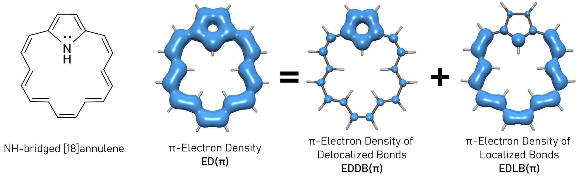
EDLB represents the density of electrons which are localized at bonds or lone pairs.

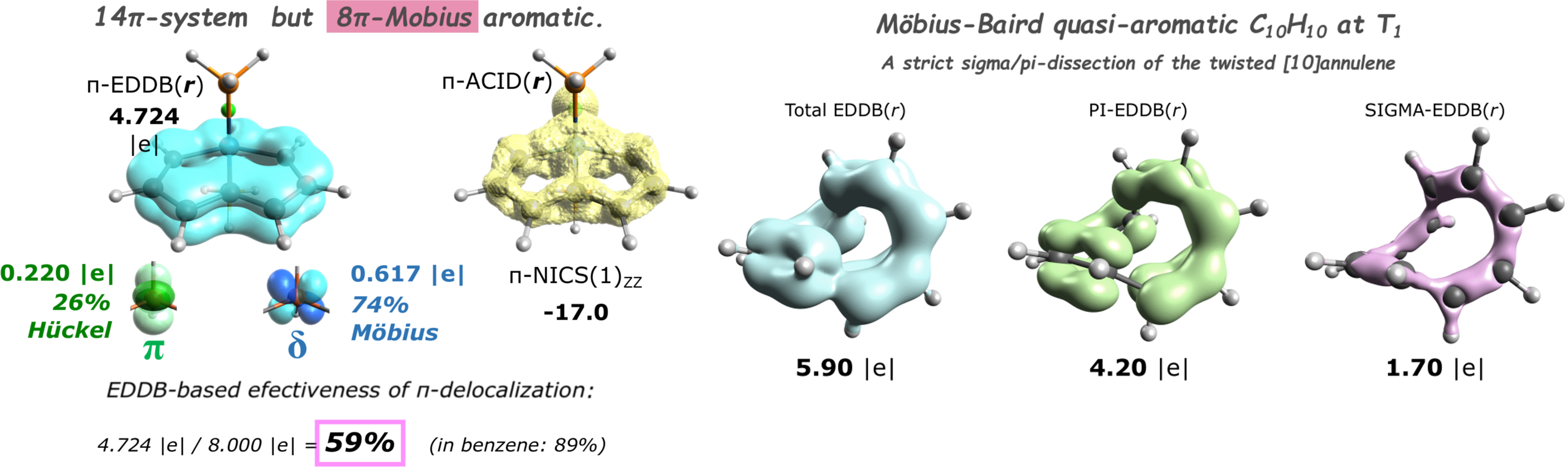
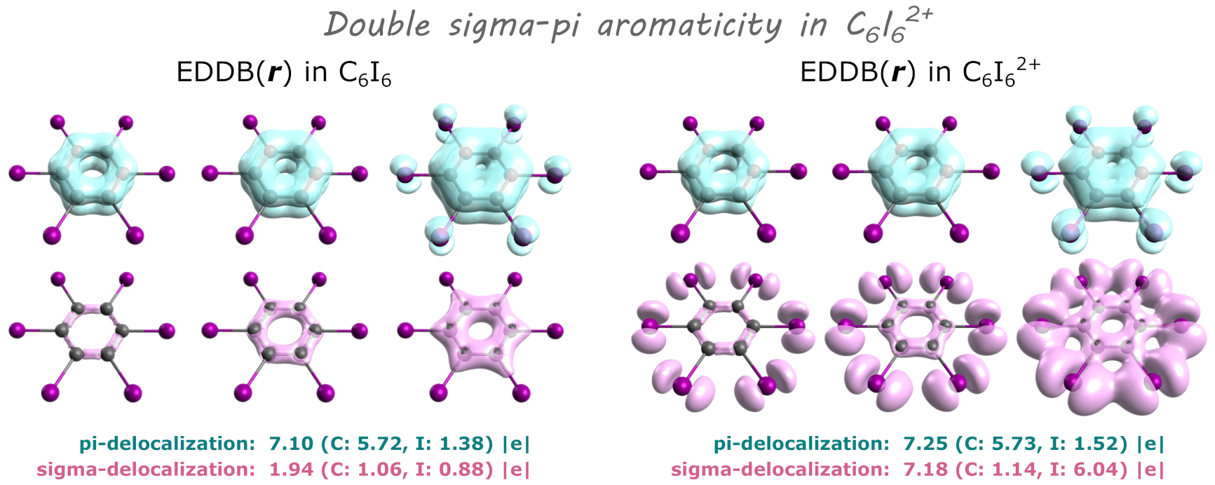
EDDB partitioning can be performed for any system including: planar and non-planar pi-extended systems, sigma-aromatics, metallaaromatics, metal clusters, 3D-aromatic systems, radicals, Möbius-aromatic systems and many more. In addition, EDDB allows for orbital-symmetry dissection (σ,π,δ…).

EDDB density comes in different variants, which you can select during calculation:

• EDDB_G – global, includes all electrons;
• EDDB_H – same as above, but excludes contribution from hydrogen atoms;
• EDDB_F – fragment, evaluates delocalization between selected atoms;
• EDDB_E – same as above, but also includes external delocalization, between selected atoms and other atoms;
• EDDB_P – pathway, evaluates delocalization along selected cyclic pathway, e.g. benzene ring;

Populations of cyclically delocalized electrons from EDDB_P are a popular aromaticity index, introduced and compared with other indices in Phys. Chem. Chem. Phys. 2017 , 19 , 28970.  URL  

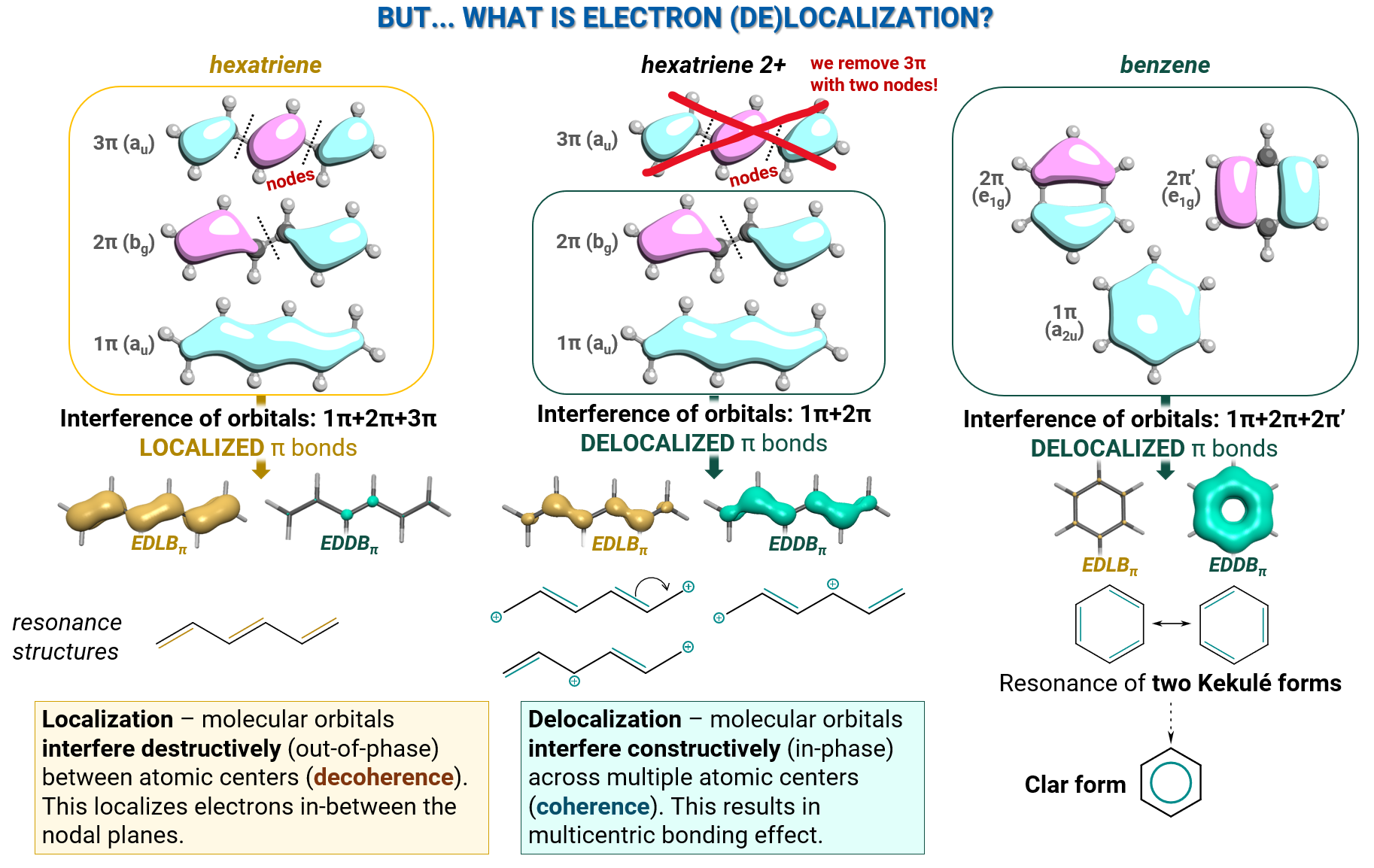
Electrons are quantum particles (fermions), whose physical properties are determined by the wavefunction. The (de)localized character of electrons bound in molecules, originates from the interference of electron wavefunctions, molecular orbitals. Their interference is determined by topology and nodal characteristics of orbitals, as illustrated below:

The last example, benzene, shows that the source of aromatic stabilization—degeneracy of energy levels in cyclic systems—is inextricably connected with constructive interference of orbitals that lead to cyclic delocalization. This is why this connection is highlighted in the first sentence of IUPAC definition of aromaticity. The cause of degeneracy and aromatic stabilization can be traced to the particle-on-a-ring analytical solutions to the Schrödinger equation (Solà, M.; Szczepanik, D. W. Pure Appl. Chem. 2025 , 97 , 1149.  URL  ) .

EDDB examples

◼Installation

Currently, EDDB is available as a free-to-use script in R language (RunEDDB).

Download links:

• RunEDDB.R   URL  
• RunEDDB.bat   URL  

The script works on Windows, Linux and MacOS. RunEDDB.R script requires free R software environment to work. Download links for Windows, Linux, MacOS are available here:   URL  

Linux installation
To install and configure RunEDDB in $HOME under Debian/Ubuntu just copy the following command and paste into Linux terminal:

The above command also installs the required R software, so after running it everything is set up.

Alternatively, you can download RunEDDB.R from the link above, put it in your $HOME directory, and define alias within .bashrc file:


Windows installation
To install and configure RunEDDB.bat under Windows 10/11 please follow the steps described in the video below:
If you installed different version of CRAN (R) please remember to modify the CRAN_VERSION variable at the beginning of the RunEDDB.bat file.

Alternatively, you can download RunEDDB.R and copy it into the folder with your .fchk and .49 input files and open the script with R software.

Other useful free software for creating EDDB visualizations include:

• Avogadro. https://avogadro.cc/   URL  
• Avogadro2. https://two.avogadro.cc/install/index.html   URL  
• IQmol. https://www.iqmol.org/downloads.html   URL  
• Multiwfn. http://sobereva.com/multiwfn/   URL  

If you use EDDB in your work please cite the original papers which introduce EDDB:

• Szczepanik, D. W.; Andrzejak, M.; Dyduch, K.; Żak, E.; Makowski, M.; Mazur, G.; Mrozek, J. A Uniform Approach to the Description of Multicenter Bonding. Phys. Chem. Chem. Phys. 2014, 16, 20514–20523 (https://doi.org/10.1039/C4CP02932A)   URL  
• Szczepanik, D. W. A New Perspective on Quantifying Electron Localization and Delocalization in Molecular Systems. Comput. Theor. Chem. 2016, 1080, 33–37 (https://doi.org/10.1016/j.comptc.2016.02.003)   URL  
• Szczepanik, D. W.; Andrzejak, M.; Dominikowska, J.; Pawełek, B.; Krygowski, T. M.; Szatylowicz, H.; Solà, M. The Electron Density of Delocalized Bonds (EDDB) Applied for Quantifying Aromaticity. Phys. Chem. Chem. Phys. 2017, 19, 28970–28981 (https://doi.org/10.1039/C7CP06114E)   URL  

◼Quick start

Below, we describe in details how to perform EDDB analysis and create visualizations using RunEDDB script and other software.

Generating input .fchk and .49 files
RunEDDB requires two input files present in current folder: .fchk and .49. .fchk is a standard formated checkpoint file from Gaussian calculation. .49 contains density matrix in NAO (Natural Atomic Orbital) basis. It is generated during Gaussian calculation if keywords in bold are included in Gaussian input file (example below):



The above calculation generates file_name.chk (you need to convert it to .fchk) and file_name.49. If you use NBO6 or NBO7 replace Pop(NBORead) with Pop(NBO6Read) or Pop(NBO7Read) and in the $NBO ... $END line add FIXDM keyword. We recommend using NBO6 or NBO7 rather than the old 3.1 version included in Gaussian, if you have access to newer versions.

Running RunEDDB in interactive mode
Linux: navigate into folder with .49 and .fchk files, then launch RunEDDB program by typing runeddb in console and press Enter. Interact with program via the terminal, it will guide you through the calculations step by step.
Windows: go into folder with .49 and .fchk files, click right mouse button and press “Open in Terminal”. This should open the PowerShell console. Type runeddb and press Enter. Follow the instructions in the interactive mode. This is also shown in the video in the "installation" section. Alternatively, you can just copy RunEDDB.R script file into the folder with your .49 and .fchk input files and open the script with R software.

Running RunEDDB from console
paste into console:

explanation of the input line commands:

• -i [files] input .fchk and .49 files
• -g, -h, -f [atom_list], -e [atom_list] or -p [pathway] selects EDDB_G,H,F,E,P variant. If you select -f or -e you have to provide the atom list,   e.g. -f 1,2,3,4,12 (or shorter -f 1:4,12). If you select -p you have to provide the ring atom list e.g. -p 1-2-3-4-5-6-1
• -d [orbital_list] (optional) list NOBD orbitals to dissect, e.g. -d 1,2,3 or shorter -d 1:3
• -od (optional) outputs EDED.fchk with dissected orbitals (from -d command). if you dissect π orbitals, you can generate the total π-electron density from this file
• -o [files] output .fchk and .out files.

if you run calculation inside bash.sh script you have to replace runeddb alias with the full command:


Analysis and visualization of EDDB results
EDDB calculation with RunEDDB outputs two files: .out and .fchk. Explanation of the .out file is provided below:


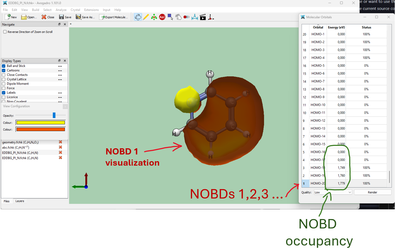
Output EDDB.fchk file contains NOBDs (which replace orbitals in the original input_file.fchk) with their occupations (which replace orbital energies in eV). Total electron density in this file is replaced with EDDB_G,H,F,E,P depending on the variant chosen. EDDB.fchk can be used to visualize NOBDs or EDDB density isosurfaces. In the example we will analyze EDDB_G results. Open EDDB_G.fchk in Avogadro or Avogadro2. NOBDs can be visualized like standard orbitals from any .fchk file. They are listed from bottom (most delocalized) to top (least delocalized) on the orbital list. Only the first 3 NOBDs are occupied, because we dissected the first 3 pi-orbitals (-d 1:3).

In general, if you want to analyze pi-electrons, dissect first 3 orbitals if you have 6 pi electrons and so on. If you are not sure, first perform EDDB calculation without the dissection, view the orbitals in the .fchk file, note the pi-symmetry orbital numbers and repeat calculation with dissection.



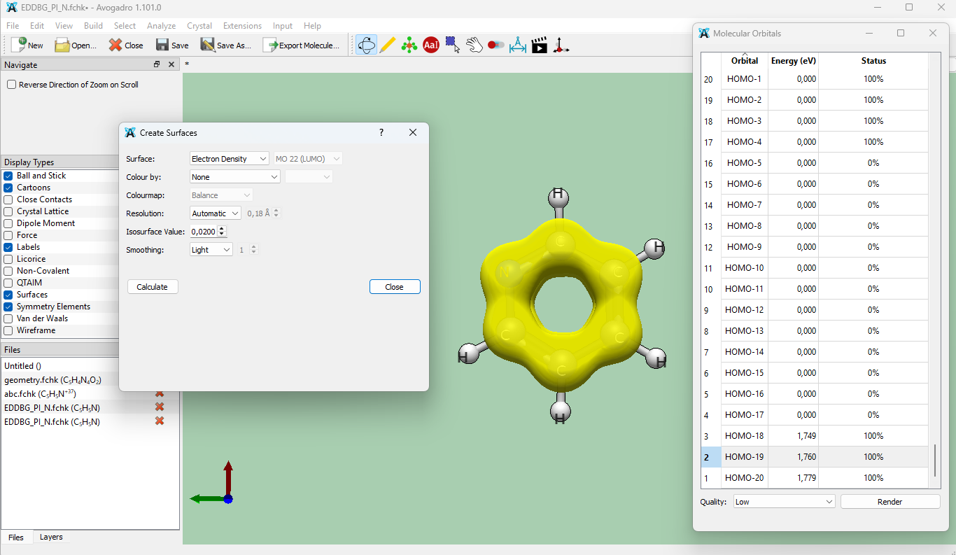
To visualize EDDB isosurface, go to Analyze -> Create Surfaces (Avogadro2) or Extensions -> Create Surfaces (Avogadro). Select Electron Density, isosurface value (typically between 0.01-0.03) and press calculate. Below is the 0.02e isosurface of EDDB_G function for pyridine:


You can generate .cube file with EDDB density using cubegen utility in Gaussian software, using the following line:

The below command generates EDED.cube using the same grid as previously generated EDDB_G.cube:

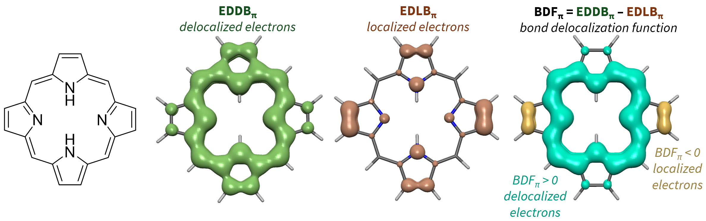
.cube files on the same grid can be subtracted, which is useful for calculating EDLB = ED − EDDB or BDF = EDDB − EDLB (BDF function:  URL  )

EDDB visualizations and analyses can also be performed in Multiwfn. However, additional modification of the wavefunction has to be done. Open EDDB_G.fchk in Multiwfn and follow the steps:

• select option 6 (Check & modify wavefunction)
• select option 30 (Exchange energies and occupation numbers for all orbitals)
• select option 1 (Exchange orbital energies (in eV) with occupation numbers).

The wavefunction is now modified, you can return (option -1) and

• visualize NOBDs (option 0), view the NOBD orbital list with their occupations (option 3)
• visualize EDDB density (option 5 Output and plot specific property within a spatial region (calc. grid data), then option 1 Electron density, then option -1 Show isosurface graph)
• and generate .cube file with EDDB density grid (option 2 after you calculate Electron density grid data).

The .cube files can be visualized in IQmol, Multiwfn or Avogadro. To visualize localized electrons, EDLB, you have to generate .cube files with total electron density ED.cube and EDDB.cube using the same grid, and then subtract .cube files: EDLB = ED − EDDB in Multiwfn program (option 13 Process grid data).

ABOUT US       PROJECTS       PUBLICATIONS       EDDB       TUTORIALS       X